
Maps: putting the Earth on paper or on screen
Learning Outcomes
By the end of this section you should be able to
- Distinguish between simple map projections
- Specify the location of a place using geographic and projected coordinate systems
- Determine distances using the scale of a map
- Recognize features indicated by contours
Many parts of this book are illustrated with maps. We use maps to show many kinds of features, typically features that vary across the Earth’s surface: the pressure and temperature of the air, the currents in the ocean, the types of plant and animal (including human) life on Earth, and the distribution of mountains and valleys. In all these types of map, we wrestle with the fact that our sheets of paper and computer screens are mostly flat, whereas the Earth is decidedly not flat. In this section we will look at the techniques, and compromises, that make maps possible.
Projections: Making the Earth look flat
The Geosphere, the solid Earth, has a surface that is round, but not exactly a perfect sphere. Because of the rotation of the Earth (and the fact that the Earth’s interior is not rigid) it bulges slightly at the Equator. It also has mountains and valleys, and other bumps and dents, that make its shape complex. To portray this shape on a flat sheet of paper or a computer screen is not straightforward. The three-dimensional Earth must be made to fit on a two-dimensional surface. This process is known as projection.
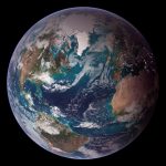
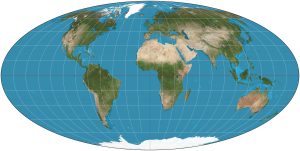
A very simple projection of the Earth approximates what an astronaut would see in a photograph taken a long distance away from the Earth, called an orthographic projection.
The orthographic projection makes it very easy to visualize the Earth’s shape, but for other purposes it’s quite deficient. Half the Earth is invisible, and near the edges the surface is very foreshortened, so that everything is very distorted. Most map projections attempt to reduce this distortion, but it’s mathematically not possible to get the round Earth onto a flat screen without distorting something.
To make a better projection it’s first necessary to imagine an ideal shape for the Earth that evens out the mountains and ocean basins. Most map projection methods assume that this shape is an oblate spheroid, a type of ellipsoid obtained by flattening a sphere in one direction (in this case the direction of the Earth’s rotation axis).

In the Earth’s case the flattening is not large – the distance between the north and south poles is is about 42 km less than the distance across the Earth at the Equator (12756 km), or about one part in 300. Most maps are made by assuming that the Earth’s shape is approximated by a spheroid known as the map datum.
![]()
WGS84 – a commonly used map datum
A simple projection can be made by wrapping a sheet of paper in a cylinder around the Earth, and imagining rays from the centre of the Earth extending out, through the features of the Earth’s surface until they hit the sheet of paper. Features are marked on the paper where these rays hit it. The paper is unrolled to make a map. Such a projection (a cylindrical projection) produces a highly distorted view of the Earth. Areas near the poles are very stretched out (because the paper is a long way from the Earth’s surface), and the poles cannot be shown.
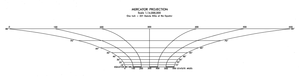
A modified form of cylindrical projection, called a Mercator projection after its first major user, decreases the distortion a little so as to perfectly preserve the angles between lines. The Mercator projection thus has huge advantages for navigation. It was extensively used by mariners who would plot a line on a Mercator projection map showing where they wanted to go, and could measure the correct compass direction for navigation directly from the map.
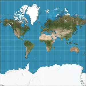
The Mercator projection is still very widely used, but it does have some disadvantages. Although it preserves angles, it distorts areas a great deal. It makes Canada and Greenland appear disproportionately large, while Africa appears disproportionately small. The north and south poles can’t be shown at all.
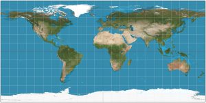
Another modified cylindrical projection, the equirectangular projection, reduces this distortion (but does not eliminate it) by portraying north-south distances using the same scale as east-west distances at the Equator. Countries near the poles still appear larger, but the distortion is not as great. Equirectangular projections make it particularly easy to plot measurements recorded in geographic coordinates of latitude and longitude (more about coordinates below), so it’s often used for computer display of data from across the globe. Because of this, in GIS programs equirectangular displays of data are often referred to as “unprojected”, although strictly speaking this is not really correct, as the Earth has to be projected to make any two-dimensional map.
Other projections, known as equal-area projections, have been devised to avoid the problem of area distortion inherant in the Mercator projection. However, these projections inevitably distort shapes and angles.
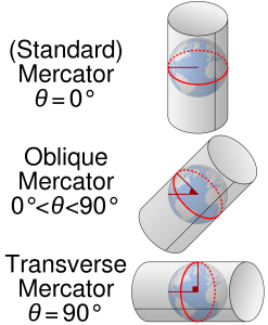
One common solution to the problem of distortion is to turn the projection cylinder so that it’s not parallel to the Earth’s axis. In the UTM (universal transverse Mercator) projection, the Mercator projection is rotated 90° and is used for a zone that is only 6° of longitude wide. The projection cylinder is rotated 6° at a time to make 60 separate UTM zones extending from near the North Pole to near the South Pole. These maps have less than 1% distortion even at the edges of the zone. They are widely used for everything from hiking to planning cities.
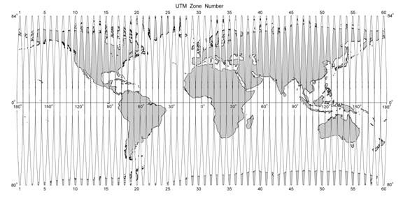
Although UTM maps are widely used for large-scale maps of small parts of the Earth, they become less useful when a map crosses two or more grid zones. Other projections are typically used for portraying large countries, continents, and the whole Earth.
Coordinates: Figuring out where you are
It’s important to be able to specify a position on the spheroid to somebody else. Two basic methods are available for this.
Geographic coordinate systems
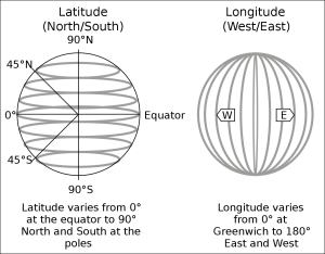
Geographic coordinate systems express position on the 3-dimensional Earth using angles. Typically these angles are measured in degrees around the Earth’s surface northward from the Equator towards the pole (latitude), and eastward from the Greenwich Meridian (longitude). Latitudes south of the Equator are either recorded as negative, or are distinguished by specifying S or N. Similarly, longitudes west of Greenwich are either recorded as negative, or are distinguished by specifying all longitudes as E or W. Notice that latitudes vary between 90° N and S, whereas longitudes vary between 180°E and W. It’s quite common for locations to be specified with latitude (north or south) first and longitude (east or west) second. (For most maps this is opposite to the convention for Cartesian coordinates on graph paper, where the X-direction is specified first.)
Example
The location of a sample of reef limestone in the Geoscience Garden at the University of Alberta in Edmonton, AB, Canada can be specified as
- Decimal degrees
- 53.28671°N
- 113.524277°W
Sometimes, instead of specifying decimal degrees as above, fractions of a degree may be specified using minutes (one sixtieth of a degree, represented with a single quote ‘ symbol), or minutes and seconds (a second is a sixtieth of a minute, represented with a double quote ” symbol). The location above becomes:
- Degrees and decimal minutes
- 53° 17.2026′
- 113° 31.4566′
- Or degrees, minutes and seconds
- 53° 17′ 12.156″
- 113° 31′ 27.397″
The first format (decimal degrees) is by far the easiest to use if you have to carry out any kind of systematic data entry or calculation using locations.
Projected coordinate systems
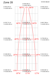
An alternative way to express position is by measuring distances on the projected (and therefore flattened) surface of the Earth. The most commonly used method is to superimpose a grid on the UTM projection, aligning it with the central north-south line (meridian) that runs through the middle of the UTM zone. The position of a point is then given by its distance from a point where the central line intersects the Equator, as a distance east (or easting, usually givern first) and a distance north (or northing, second). However, to avoid negative numbers, the central meridian is given an easting of 500,000 m, and, in the southern hemisphere, the Equator is given a northing of 10,000,000 m. This means that eastings are always six-digit numbers but northings are seven-digit numbers. When using UTM coordinates for large areas, it’s important to specify which zone you are working in.
![]()
Example
The location of the sample of reef limestone in the Geoscience Garden at the University of Alberta in Edmonton, AB, Canada can be specified as
- UTM Zone 12 North
- Easting 332687
- Northing 5934048
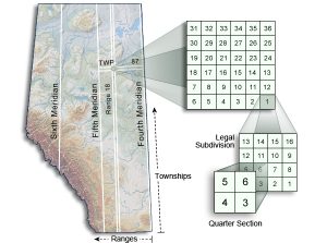
Other coordinate systems
Before the widespread use of UTM coordinates, other methods were used on projected maps of the Earth’s rounded surface. A variety of schemes were devised during the colonization of North America and other parts of the world by European settlers in the 19th century, often with the aim of documenting imposed European-style land ownership in previously undivided indigenous lands. One such scheme is the Dominion Land Survey of western Canada, which divides the spheroid into approximate squares 1 mile on each side. This grid is numbered westward in ranges and northward in townships. Because the divisions are measured from “baselines” that are lines of latitude and longitude, the subdivisions are only approximately square, and E-W “correction lines”, that offset the grid, are inserted at 4-mile intervals to cope with the curvature of the Earth. Despite these approximations, the Dominion Land Survey is still widely used in western Canada for land and resource management.
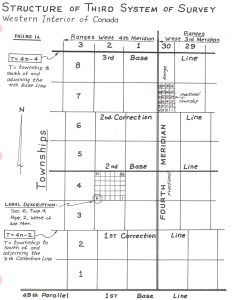
https://www.alsa.ab.ca/Portals/0/Images/Surveys%20in%20Alberta/structure.jpg?ver=HNkQB0BrjAcs4ReO1nc8cw%3d%3d×tamp=1610061596049
![]()
Example
The location of the sample of reef limestone in the Geoscience Garden at the University of Alberta in Edmonton, AB, Canada, would be specified as
- West of the 4th meridian
- Township 50
- Range 25
- Section 1, 1142 ft W, 1220 ft N of southeast corner
Scales: Fitting the Earth on your screen
Maps are inevitably scaled. A map that was as the same size as the landscape you were living in would be no use at all! However, the amount of scaling can be enormously variable. A large-scale map might be a plan for the construction of a single house. The maps earlier on this page that compress the whole Geosphere onto a computer screen are examples of small-scale maps.
The scale of a printed map can be presented in a number of ways.
Verbal scales
Perhaps the easiest to grasp is a simple equivalence:
2 cm = 1 km or “two centimetres to one kilometre” or
“One inch to one mile”
In each case the smaller distance (usually given first) is a distance on paper, that corresponds to the larger distance (usually second) on the real Earth.
Verbal scales are easy to grasp provided everyone is familiar with the units. Many older maps use unfamiliar units, and units in different languages. For example, older property maps could be at a scale of one inch to 40 chains, or one hand to 16 furlongs[1]. For this reason, more universal ways of representing scale have been devised.
Representative fraction
A representative fraction is a statement of how many times smaller a map is than the real world. It may be represented as an actual fraction:
1/50,000
or more usually with a colon as separator:
1:50,000
which is read “one to fifty thousand” in English but which works well in numerical regardless of the language of the user.
It’s important to note that the representative fraction is independent of units. The scale 1:50,000 is certainly more convenient when using metric units based on multiples of ten. It’s actually equivalent to the example 2 cm = 1 km in the previous section. However, the ratio applies to anything, so on such a map 1 inch would represent 50,000 inches (a little over three quarters of a mile), and one cubit would represent 50,000 cubits!
The other example above (1 inch = 1 mile) translates to 1:63,360.
It’s important to remember that these numerical scales are fractions. Therefore, the larger the number in the denominator[2] the smaller the scale of the map.
Scale bar
The above two methods of specifying the scale of a map work well for maps printed on paper, but many maps are now displayed on screens, not printed on paper. This presents problems of specifying the scale, because the person who makes a map has no control over the size of the screen on which it will be displayed. For these purposes, and for any map that may be enlarged or reduced, it’s best to use a scale bar: a line representing a known distance. For example, in the case of a 1:50,000 map the scale bar might be 2 cm long and it would be labelled “1 km”. Scale bars do not have to be a single unit long. A 1:50,000 map might have a scale bar 8 cm long, labelled “4 km”. In such cases it’s common to put ticks or black and white boxes to show single kilometres.

The advantage of a scale bar is that if the map is enlarged or shrunk to fit on a screen, the scale bar undergoes the same change and remains correct, whereas verbal scales or representative fractions become invalid as soon as the map is reprojected onto a screen.
Scale variation
Because of the problems of getting a spheroidal Earth onto a flat surface, no projected map has absolutely constant scale. For large scale maps this is not usually a huge problem for normal purposes. For example, within a UTM zone the scale varies by lest than 1%. However, for maps of the whole Earth, and particularly maps in Mercator projection, the scale bar must specify at what latitude it is to be used. For some maps a more complex diagram showing the relationship of scale to latitude is used.
Contours: displaying variables
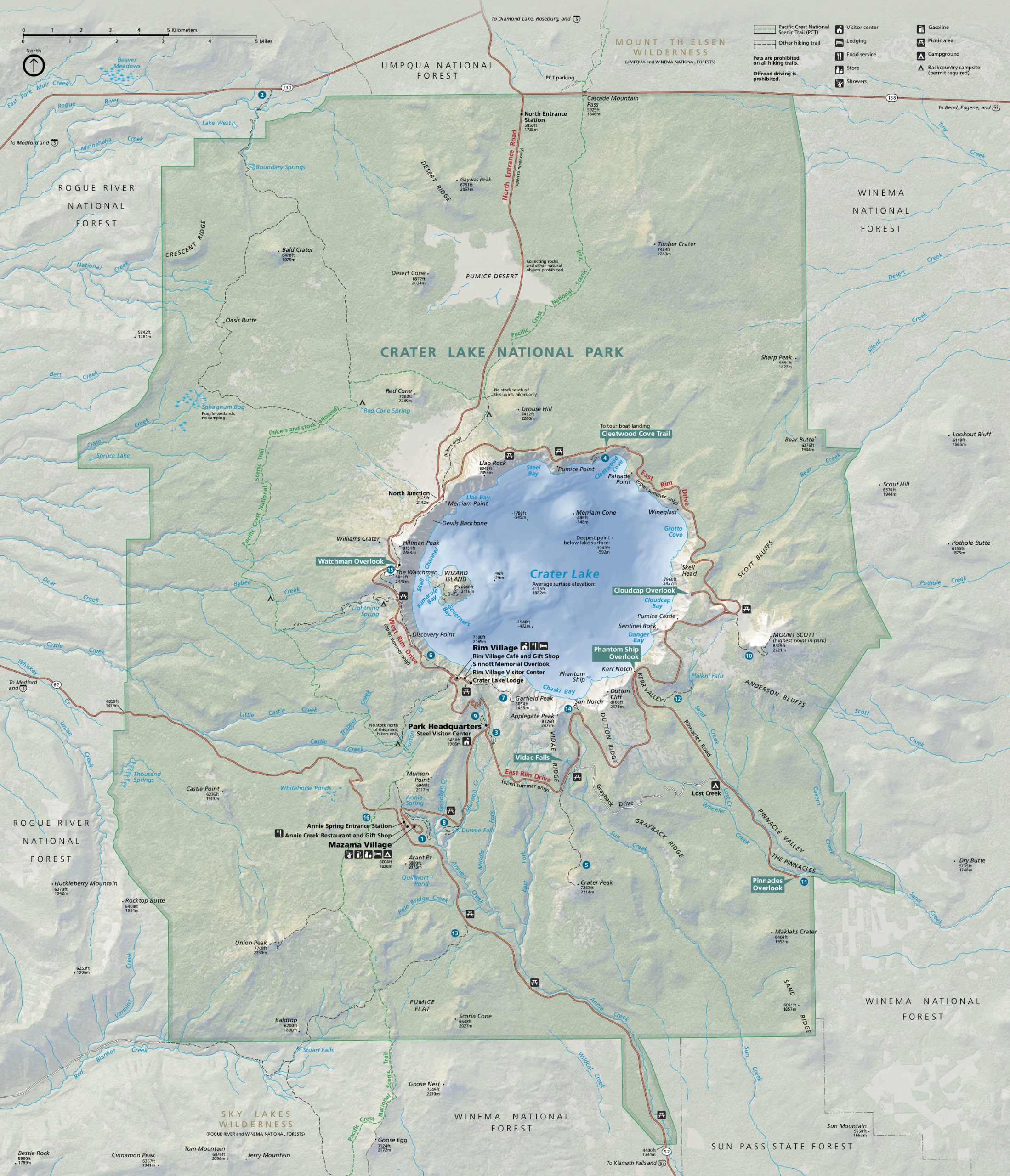
Topographic contours
Historically, surveyors would travel the landscape and measure the elevation (above the geoid, or mean sea-level) of as many points, called spot heights, as possible. Modern methods such as LiDAR[3], using lasers, have made possible the generation of many more survey points in a point cloud or a digital elevation model, but the principle is the same. Point clouds are particularly difficult to understand when viewed.
Topographic contours make point data easier to understand. Each contour is a line separating higher and lower parts of the landscape.[4] For example, the 1000 m contour might have points measured at 1001, 1009, 1003 on its “high” side and 998, 993 and 999 on its “low” side. If by chance a point is exactly 1000 m above sea level, the contour will pass right through it.
By drawing contours at standard elevations all over a map, it’s possible to simplify a point cloud or a set of spot heights into a picture that’s reasonably easy to understand. The picture can be made even more informative by adding colours to represent different ranges of elevation.
The spacing of contours indicates the slope of the land. Widely spaced contours indicate gentle slopes, whereas closely spaced contours indicate steep gradients. If two or more contours coincide on a map, this indicates a vertical cliff.

Topographic contours should be labelled with numbers indicating their elevation. On maps with many contours it is common to number only every fifth contour (for example) to avoid cluttering the map. However, under these circumstances it is sometimes necessary to indicate which is the “high” and which is the “low” side of each contour. Typically the “low” side is marked by a “hachure” or tick-mark. This is particularly necessary for closed contour loops where there isn’t room for numbers. In some maps only closed depressions are marked with hachures. Closed contours without ticks are assumed to be peaks.

On some maps, gradients are “hillshaded” using the contour spacing and orientation, to create an illusion of a 3D surface. Note, however, that the direction of the simulated illumination can affect the visual perception of slopes.
Contour maps for point data are non-unique, and represent a hypothesis for the shape of the landscape. Usually the simplest, smoothest set of lines is drawn, provided that it is consistent with every data point.
Other types of contour
Contour maps of the sea floor are commonly numbered with depths below mean sea-level. Such maps are known as bathymetric contour maps.
In principle, any quantity that varies geographically can be represented by a contour map. In some cases the contours have special names. In this book, you will encounter maps that are contoured according to the value of pressure (isobars), temperature (isotherms) and many other measured values (for example concentrations of salt in the ocean) that are generally termed isopleths. In all these cases, closely spaced contours indicate that the measured quantity changes rapidly with position. Widely spaced values indicate lower gradients of the measured quantity.

- A chain, still used for measuring land in some jurisdictions, is 22 yards; a hand (still used for measuring horses) is 4 inches; a furlong (also familiar to horse-riders as a common measure for race tracks) is 10 chains or 880 yards, or one eighth of a mile. ↵
- The denominator is the number after the : or / symbol. ↵
- Light Detection and Ranging) ↵
- Contours are sometimes defined as "lines joining points of equal elevation". However, this definition is less helpful to novices in contour threading as there are often no points of equal elevation on a map to be contoured. Also, when contour threading it's sometimes easy to draw a line that does join points of equal elevation but which fails to separate higher and lower points properly; higher or lower points appear on both sides of the line. Hence the definition given here, of a line separating higher and lower elevations, is much better. ↵
In map making (cartography) projection is the process that transforms the 3-dimensional Earth onto a 2-dimensional page or computer screen.
global positioning system
world geodetic system 1984
Geographic information systems
Universal transverse Mercator
A data set of arbitrarily located points, each of which is represented by three coordinates, typically representing an easting, a northing, and an elevation
A data set of points that are equally spaced in two horizontal directions (usually E and N); each point is associated with an elevation.
