
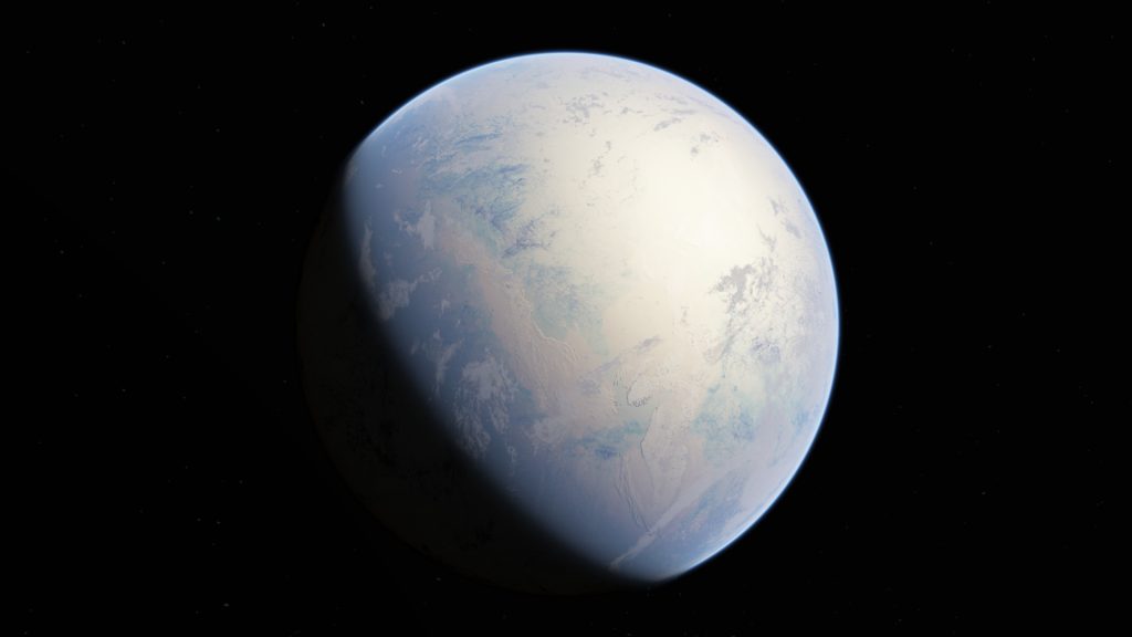
24 Climate and Climate Change
Britta Jensen; Jeff Kavanaugh; and John W.F. Waldron
This chapter is a final draft; glossary entries and cross-references have yet to be completed.
In this chapter, we will look at the science of climate change. Although the study of climate is part of atmospheric science, our understanding of climate involves all the Earth’s spheres, particularly including ocean circulation, energy capture by the Biosphere, and geologic time.
Learning outcomes
By the end of this chapter, you should be able to:
- Explain how past climate conditions are reconstructed using proxies;
- Describe natural variability of climate over long and short-term scales;
- Explain the principles of feedback and forcing, including positive and negative feedback, fast and slow feedbacks;
- Describe natural controls on climate including tectonics, solar and orbital forcings;
- Explain climate sensitivity and how it is used to predict future surface temperatures;
- Describe the main sources of greenhouse gases and their effect on global average temperatures, glaciers, sea ice, sea level and oceans.
Weather and climate
The terms weather and climate are sometimes used interchangeably, but they have quite different meanings. Weather describes the state of the atmosphere at a single moment in time, and often at a single place. As we have seen in the section on weather, the atmosphere is extremely variable, changing on a daily basis in most parts of the world.
Climate is averaged weather. How long do we have to average weather before we can call it climate? The answer is certainly at least a year, and in most cases several years. A common averaging interval for climate studies is 30 years.
The choice of averaging interval is important. In climate studies undertaken in the 20th century if was often assumed that climate was constant. Therefore, the only factor to be taken into consideration was choosing an averaging interval long enough to smooth out random changes between years.
Since the recognition of rapid, human induced (or anthropogenic) climate change, the choice of interval has become more difficulty. If too long an averaging interval is chosen, recent, rapid anthropogenic changes may be missed. If too short an interval is chosen, short term effects like the El Niño southern oscillation (ENSO) may unduly affect the result. In many cases, 30-year averages still work, but for the documentation of recent anthropogenic climate change, sometimes 10-year or even 5-year averages are used.
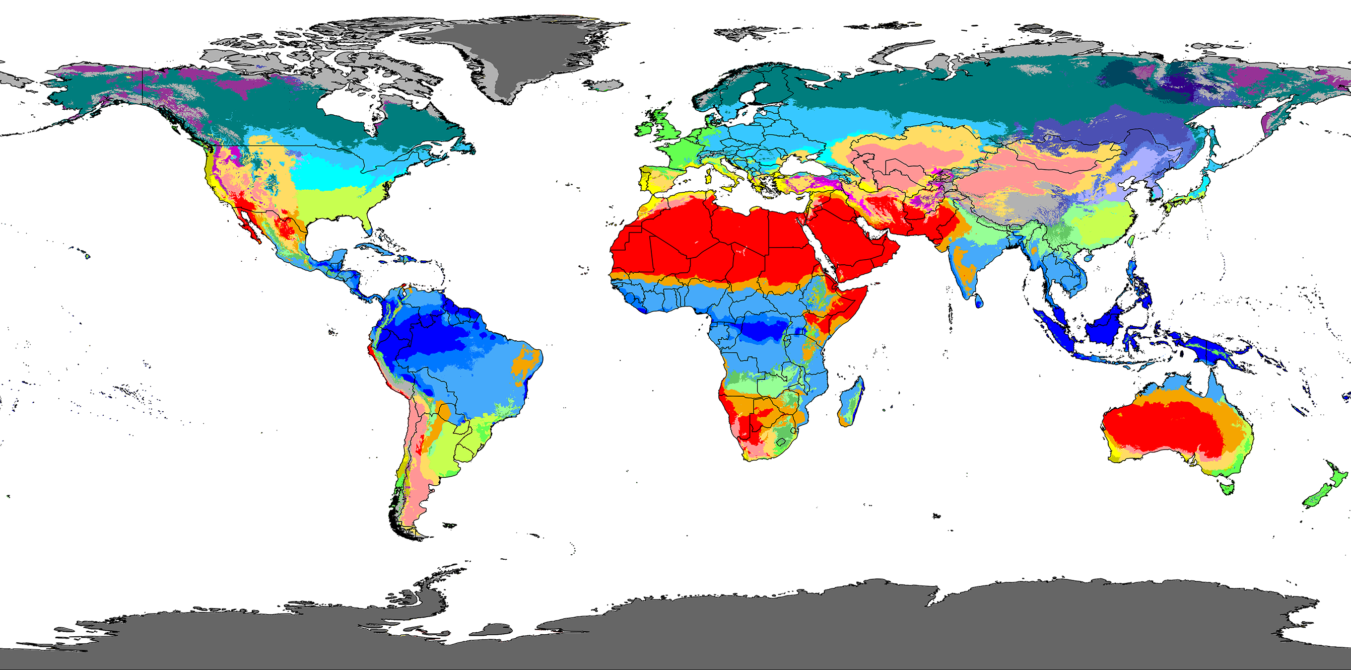
Climate has a strong impact on the biosphere. Over geologic time, organisms have evolved adaptations to particular climatic conditions, resulting in the many biomes that are distributed over the surface of the Earth. As a result, maps showing climate zones are quite similar to those showing biomes.
Recording climate change
Weather-recording instruments (thermometers, barometers, etc.) have been collecting data for a few centuries, but the record only becomes sufficiently precise for understanding climate around 1880 CE[1]. Before that we don’t have direct measurements of temperature, so we have to use proxies: a proxy is some type of information that is not a direct measurement of weather or climate, but which can related to climate in some way.
Climate proxies: measuring climate of the past
Historical proxies
Many past peoples have recorded information that allows inferences to be made about climate. Examples include:
- Paintings and drawings that show the weather at the time they were created. For example, historical artworks show that the River Thames in England would freeze over during a period of time known as the little ice age roughly from 1400 to 1850 CE.
- Oral histories and traditions telling of changes in the landscape. For example, Mi’kma’k traditions may record the first entry of tidal water into the Bay of Fundy in Atlantic Canada following the end of the last ice age[2].
- Written descriptions in both non-fictional (e.g. newspapers) and even fictional writings that are set it real places.
- Dates of first freezing or thawing of lakes, and the extent of sea ice, collected in the course of fishing.
- Records of harvest yields of crops, fishing catches, and even associated human variables like the market prices of food commodities, which respond to good and poor harvests.
Typically these records provide qualitative information about the direction of change (warmer or colder), and may be represented by indices (e.g. a 5 point scale from very dry to very wet) but not quantitative information (e.g. temperatures in degrees).
Biosphere proxies
Records of growth
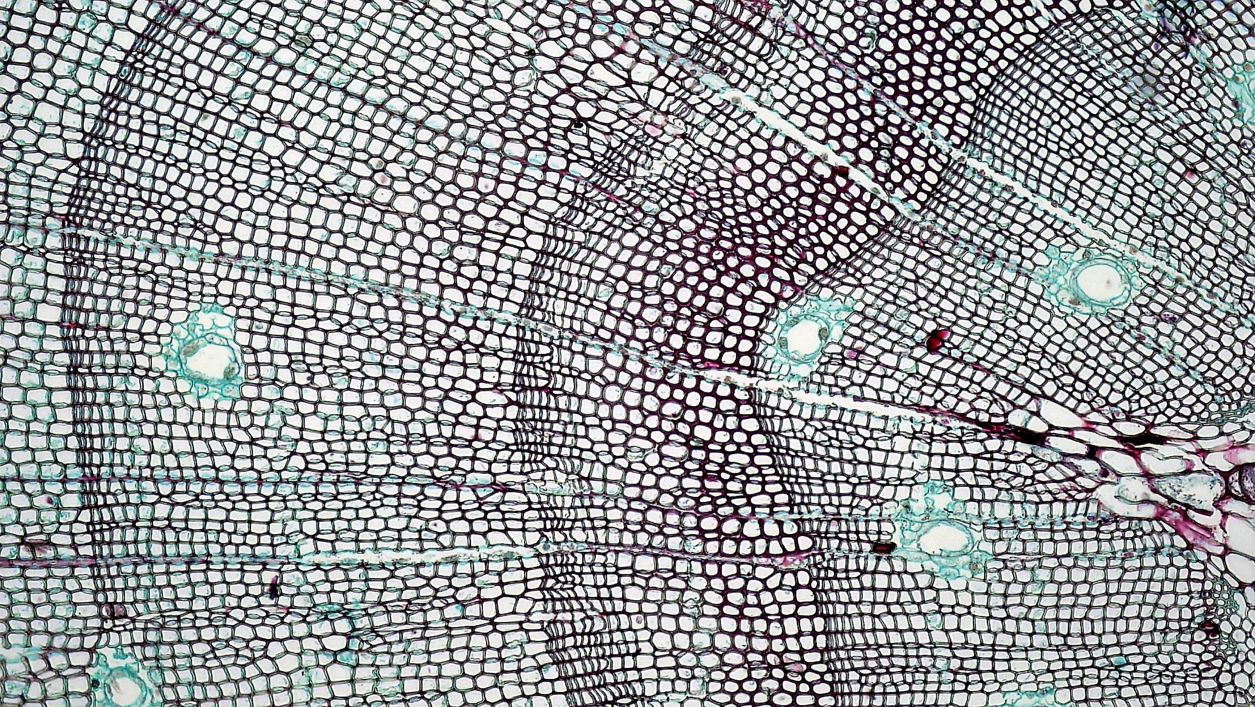
In the section on geologic time, the use of tree-rings to count years is described. The same tree rings, once their age is known, can provide information about climate change.
One tree ring records the growth of a tree during one year. The width of each tree ring is determined by factors such as the temperature, the amount of precipitation, and the length of the growing season. Which of these factors is most important depends on which one provides the greatest limitation to growth. For example, in cold temperate climates where there’s plenty of water, the main control may be the length of the growing season. On the other hand, in a warm temperate or tropical environment, the availability of water may be the main limiting factor, so wetter years (which in many climatic zones also tend to be warmer) produce wider growth rings.
Once these factors are understood, it is possible to compare the tree rings developed during the last 150 years of instrumental records to see how they respond to year by year changes in temperature or precipitation. The older tree rings may then be used as proxies to provide estimates of conditions before the start of modern weather records.
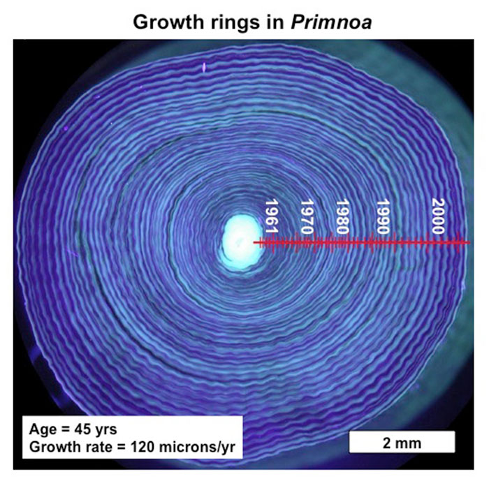
Growth bands in coral in the oceans can be used in a similar way.
 Species change
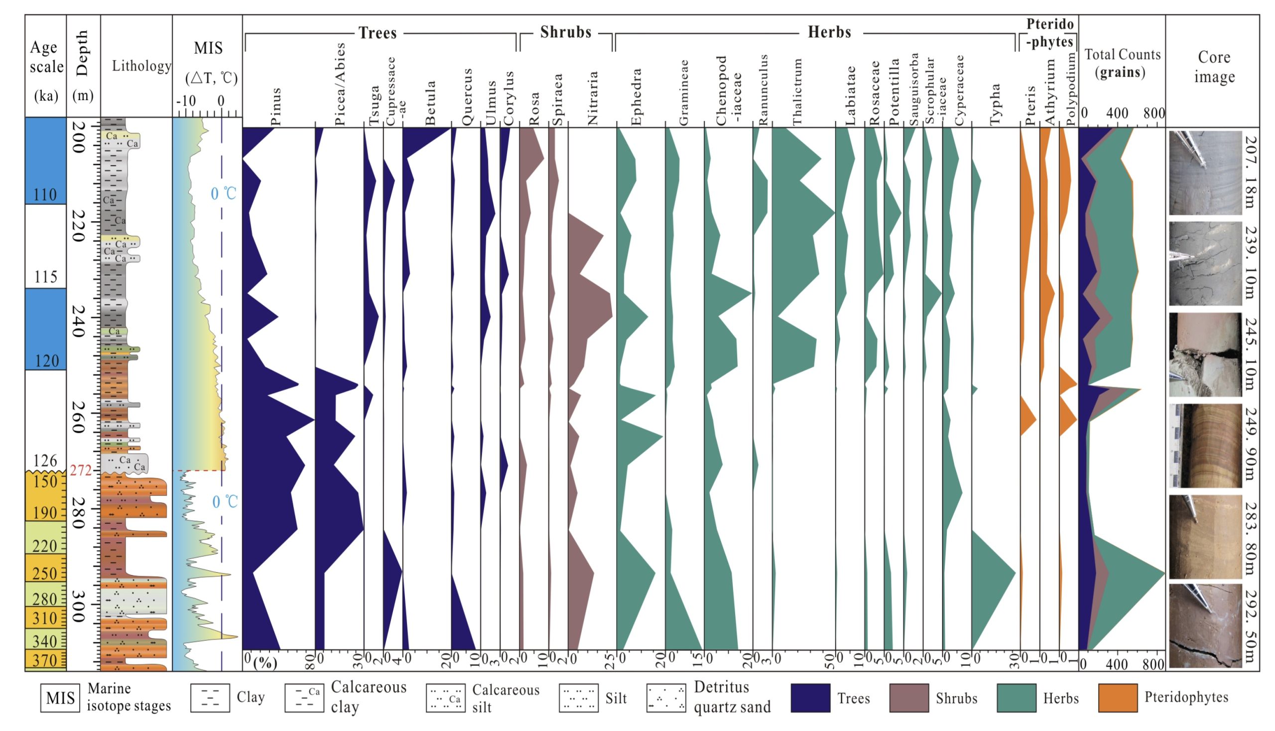
Many modern species live in ecological niches that are defined by climate – particularly temperature and the amount of precipitation. Layers of sediment, particularly fine-grained muds and oozes deposited in lakes and in the deep sea, may provide almost continuous records of sedimentation, and may capture the remains of organisms as fossils. The changing species preserved may provide information about climate change.
Typically, this work has to be done with microfossils which are abundant in fine-grained sediment, particularly in cores – narrow cylinders of sediment recovered from lake beds or the sea floor. Larger fossils (macrofossils) are not usually abundant enough to provide a detailed record.
On land, lake sediments are typically sampled for pollen grains, which show enough variation for plant species to be identified. These identifications may provide information about variations in temperature or rainfall that led to the replacement of one species by another in the land surrounding a lake.
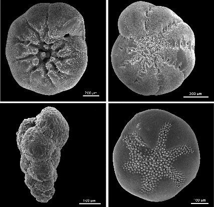
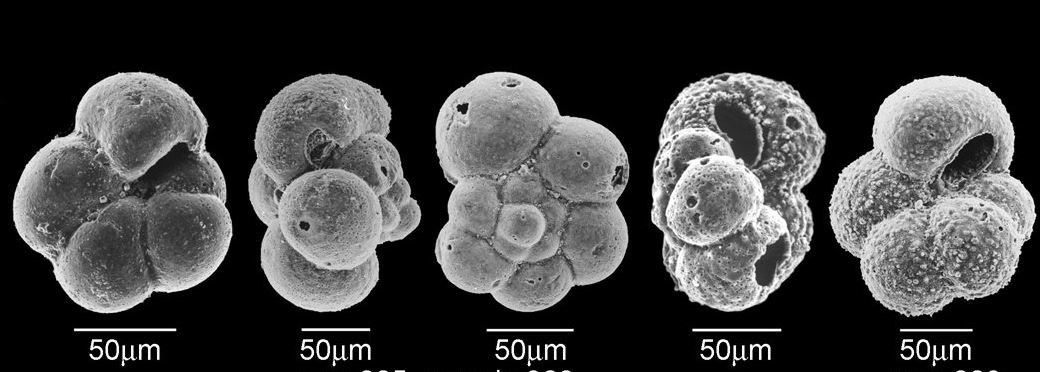
In the ocean, microfossils like Foraminifera (microscopic planktonic animals with calcium carbonate shells) may provide comparable information.
These types of evidence are most easily used in recent parts of geologic time — the last few million years. Going back further, interpreting the record becomes more difficult because evolutionary change may have occurred since the sediments were deposited. If the species present are different from modern species, it’s less easy to be sure that their response to environmental factors was the same as is observed at the present day. Furthermore, a change in the fossil record may occur because of evolution of new species, rather than because of responses to environmental change.
Fossils are still useful as indicators of climate change in earlier parts of the sedimentary record. However, isotopic proxies become more useful as indicators of climate change.
Isotopic proxies
Isotopes are variants of an element characterized by different numbers of neutrons in the atomic nucleus. Isotopes of a given element have the same number or protons and electrons, so their chemical properties are virtually identical, but their physical properties are different because they have different atomic weights.
For example, many isotopes are unstable and cause radioactivity. Radioactive isotopes are used in the measurement of geologic time. In contrast, studies of climate typically use stable isotopes — those that do not spontaneously decay – of light elements like hydrogen, carbon, or oxygen.

For example, the element oxygen (atomic number 8) exists in three stable isotopes. Oxygen-16 (16O) is by far the most abundant, and oxygen-17 (17O) is very rare, but oxygen-18 (18O) makes up a measurable amount (about 0.2%) of all natural oxygen. Because its mass is significantly heavier than oxygen-16, it behaves slightly differently. For example, a water molecule that contains 18O is significantly less likely to evaporate than one containing normal 16O, so when water is evaporated from the oceans, the water vapour tends to have less 18O than the oceans, while the water that is left behind has a slight excess of 18O. Glaciers on land are entirely made from snow that has formed from atmospheric water vapour, so they inherit the lower content of 18O from the water vapour. At times in the past when glaciers have been growing, the concentration of 18O left behind in the oceans has risen. Conversely, when glaciers melt, 18O values in the oceans change back to normal.
The changes are small, but routinely measurable. The deficiency or excess of 18O in a sample is measured in parts per thousand above or below standard ocean water. The resulting value is called δ18O (delta oxygen-18), and provides a detailed track of the growth and decline of ice sheets over the last few hundred thousand years. It can be measured from the calcium carbonate in the shells of Foraminifera and other plankton, and can also be directly measured in cores of glacier ice.
Similar changes affect the distribution of hydrogen isotopes. Hydrogen-2 or 2H is known as deuterium (D) so the corresponding value is δD. Its value rises and falls in step with that of 18O. Like δ18O, δD can be directly measured in glacial ice cores that go back, in Antarctica, about 800,000 years.
In the most recent samples, where we have direct measurements of temperature, it’s possible to calibrate the variation of δ18O, and δD with temperature. Therefore, these isotopic values can be used as proxies to generate temperature estimates going back to times before instrumental records are available.

Atmospheric samples
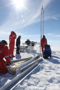
Ice cores provide additional information on climate change, beyond their content of stable isotopes. As glacier ice forms from snow, air bubbles remain trapped between the former grains of snow. Up to 10% (by volume) of glacier ice may be trapped air, and that air provides a sample of conditions near the glacier surface at the time the air became trapped. Air bubbles in ancient ice (up to 800 ka in antarctic ice cores) can be sampled and analysed to obtain data on how the proportions of atmospheric gases have varied through time.
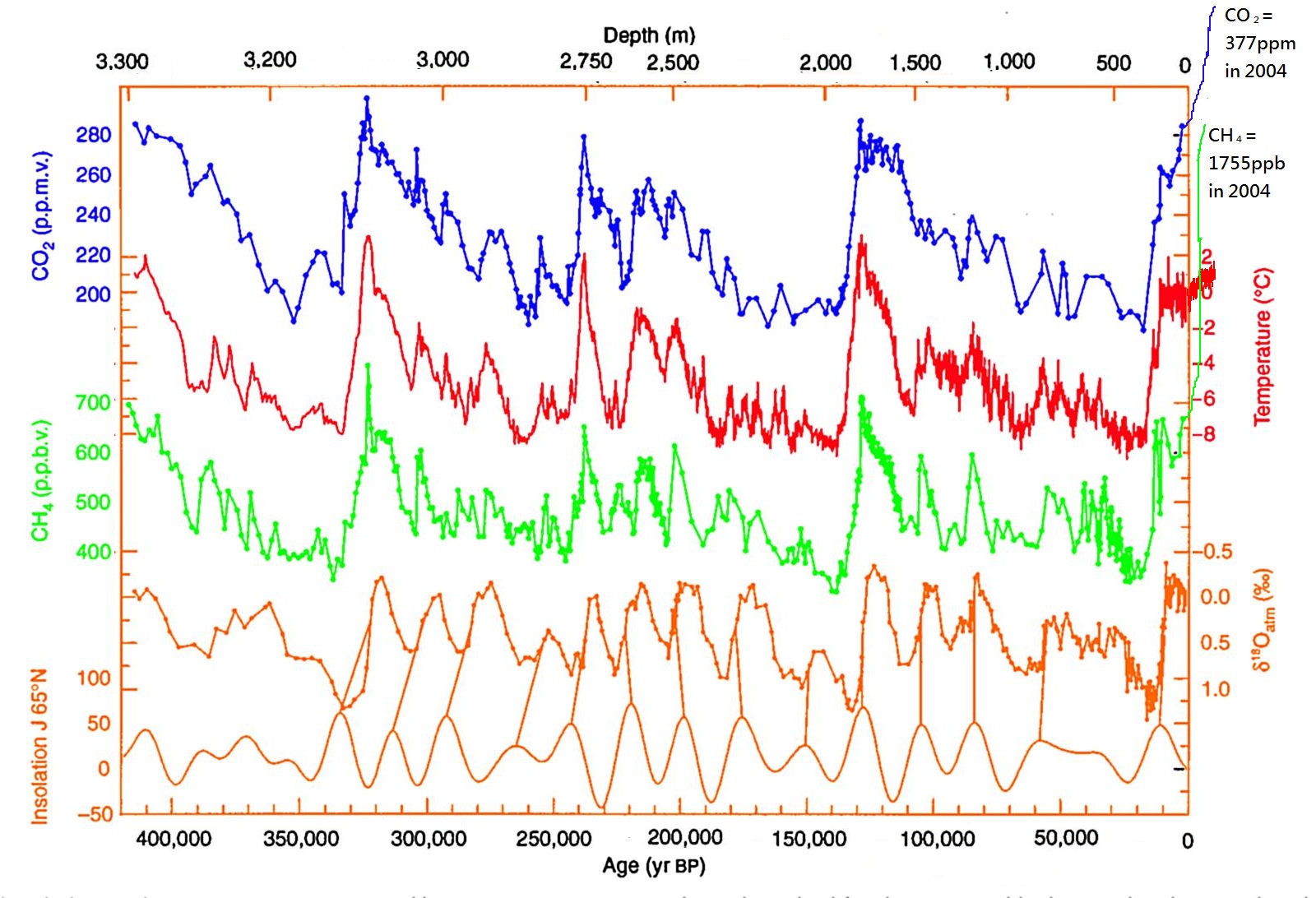
The ice-core records of carbon dioxide and methane trapped in air bubbles show strong correlation with temperature proxies, showing that both gases decreased in abundance during cold intervals with abundant glaciers, and increased in abundance during interglacial periods (such as the one we are living in at the present day).
The fluctuation in carbon dioxide varies from a low of around 170 ppm during glacial intervals, to a high of around 280 ppm during interglacial times. That value, 280 ppm, was typical of atmospheric carbon dioxide from the end of the last glaciation, around ~10 ka, until about 1750 CE, when the atmospheric concentration of carbon dioxide began to rise in response to the burning of fossil fuels during the industrial revolution. Current values are around 415 ppm, higher than at any time during the ice core record of the last 800,000 years.
The record of climate change
So what do the climate proxies tell us about Earth’s climate history? The story is quite difficult to reconstruct for at least the first half of Earth history up to the end of the Archean. Conditions were sufficiently different that most of the proxies were depend upon are not applicable. Later in Earth history the record becomes clearer, and for the last few million years there are increasing amounts of reliable data, particularly from ice cores.
Changes over millions to hundreds of million years
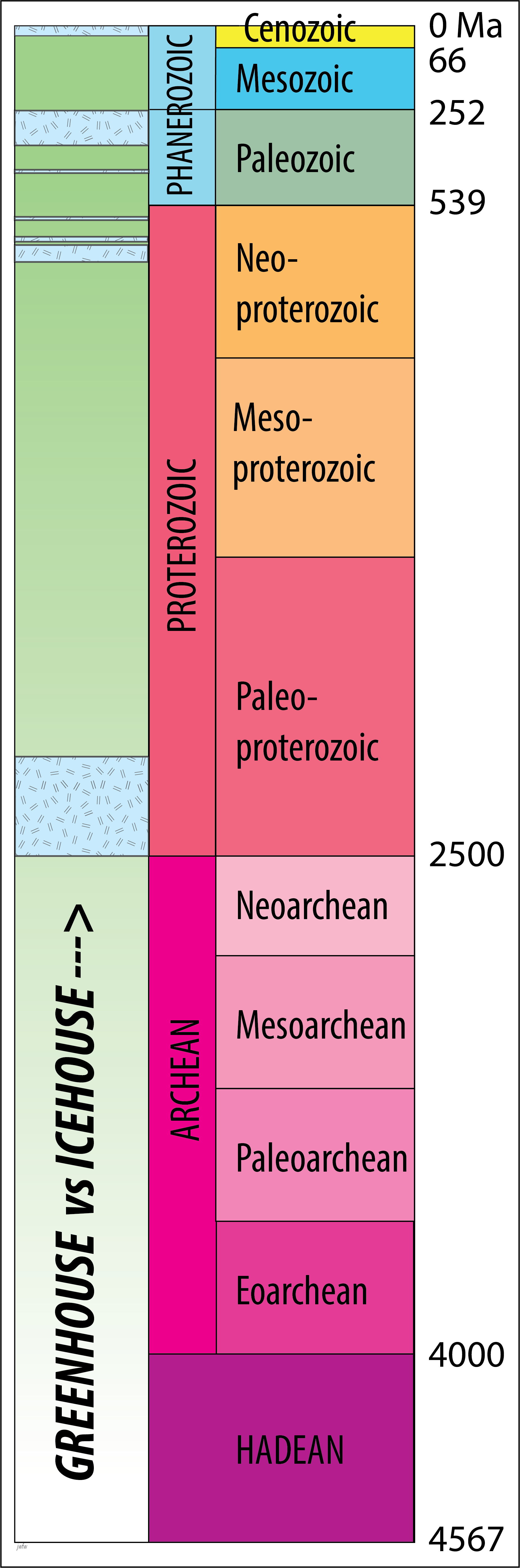
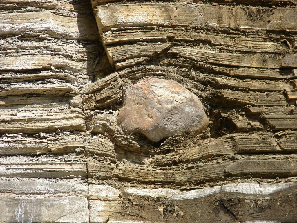
Glacial depositional and erosional features are our main evidence for climate change during the Proterozoic Eon. Evidence for glaciation tends to be concentrated in certain parts of the geological record, leading to the idea that the Earth alternates between greenhouse conditions — without significant ice sheets — and icehouse conditions, during which ice sheets advance and retreat relatively rapidly, on a scale of tens to hundreds of thousands of years.
The earliest evidence for icehouse conditions comes from tillite (lithified till) in a unit of rocks called the Huronian supergroup, in central Canada, deposited between 2.5 and 2.2 Ga in the early Proterozoic Eon.
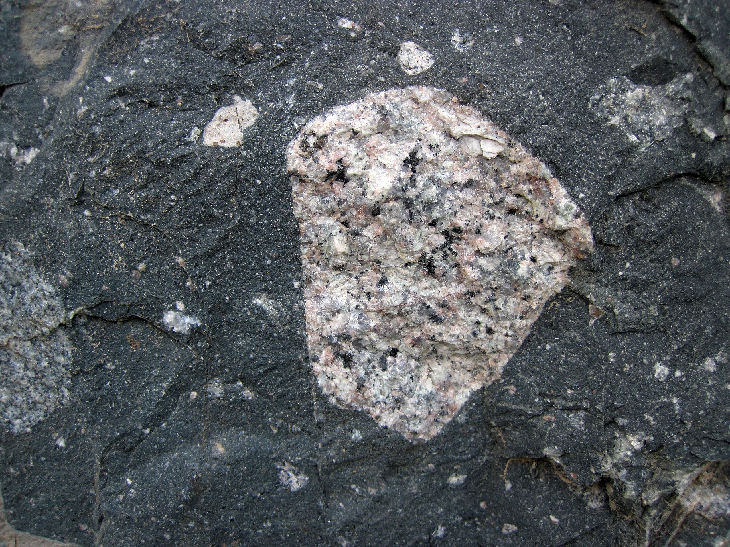
During this long interval, it appears that shorter glacial and interglacial periods alternated, as ice sheets advanced and retreated.
No more definite glacial deposits are recorded in the middle part of the Proterozoic, a greenhouse episode, but in the late Proterozoic, a series of glacial events is again recorded, indicating that icehouse conditions returned. The principal events produced deposits of tillite and other glacial features around 715–680 Ma, 650–635 Ma, followed by a final ice advance at 580 Ma. During several of these events, glacial deposits are found in rocks that show nearly horizontal magnetic inclination, indicating that they were deposited close to the equator. This suggests that for some of the icehouse interval, the Earth entered a snowball Earth state, where increased albedo led to runaway cooling, and much of the Earth’s surface became covered by ice.
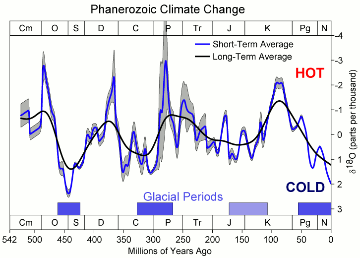
The record is a little more detailed during the Phanerozic Eon, and oxygen isotope data are available for much of this time. However, their interpretation is challenging, especially for long-term changes on a scale of 100 Myr or more, because other factors than temperature may have affected the amount of 18O in the oceans. Nonetheless, the isotopic record is in general agreement with the record of deposited till.
The first significant Phanerozoic glacial event was around 445 Ma, and was associated with widespread extinction of species, probably due to climate change. It seems to have been short lived, and may not signify that icehouse conditions were established.
A much more protracted icehouse period occurred between 360 and 255 Ma, in the late Paleozoic Era, during which time there is extensive evidence of glaciation in the continents that formed the continent Gondwana — modern South America, Africa, Antarctica, India, and Australia — which lay over the South Pole, during the time that Europe and North America lay in the tropics where coal was formed from peat deposited in the tropical rain forest biome. During this time, there was once again repeated advance and retreat of ice sheets, associated with global rises and falls of temperature and sea-level.
The Mesozoic Era corresponded generally to greenhouse conditions. However, during the Cenozoic Era, starting about 50 Ma, the climate became steadily colder, leading to the icehouse state in which we live at the present day. The Antarctic ice sheet probably started to form around 45 Ma. Cooling escalated around 34 Ma, which also coincided with a major extinction event. During the latest parts of the Cenozoic Era, increasingly wide climate fluctuations, combined with a general cooling trend, established an alternation between glacial and interglacial periods, considered in the next section.

Thousands to hundreds of thousands of years
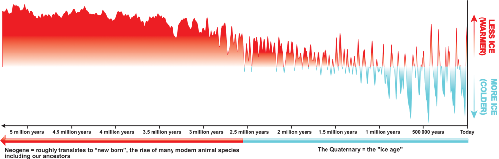
Climate fluctuations became increasingly extreme, leading to clearly recognizable glacial and interglacial episodes, occurring on time scales from tens to hundreds of thousands of years. This phenomenon became most apparent, based on the record of stable isotopes, at about 2.6 Ma, at the start of the most recent period of the Cenozoic Era, known as the Quaternary Period.
For about the first half of the Quarternary Period, these climate fluctuations took place with a cyclicity of about 41,000 years (corresponding to the Milankovitch obliquity cycle). However, as the climate grew steadily colder (on average), the cycles lengthened and widened. During the latter half of the Quaternary Period, the dominant cyclicity controlling glacial and interglacial conditions appears to have been the ~100,000 year eccentricity cycle. Smaller scale 23,000-year cycles, corresponding to the precession of the equinoxes are superimposed on the longer-term patterns.
Ice-core records show a clear match between the records for oxygen and deuterium isotopes in ice, and the records of carbon dioxide and methane in air bubbles, suggesting that all four proxies are recording the same climate fluctuations. For the last half million years there has been a clear pattern of very rapid temperature rise at the end of a glacial interval, followed by slow and stepwise cooling as the Earth cools back into a glacial episode. In the most recent of these cycles, following the last glacial maximum around 20 ka, climate warmed rapidly between 12 ka and 10 ka, by which time Earth had entered the warmest part of the interglacial period. Gradual cooling has followed since around 6 ka, continuing to historical times around 1800 CE, when the impact of anthropogenic carbon dioxide started to be felt.
Historical changes
During the “common era” since about 2 ka, we have much more detailed records from proxy data such as tree rings and historical accounts, in addition to data from stable isotopes, and it is possible to resolve changes in climate on the scale of decades to centuries. The climate curves are quite “messy” with superimposed patterns that are difficult to resolve into regular cycles. In a later section we will look at approaches to explaining these fluctuations.
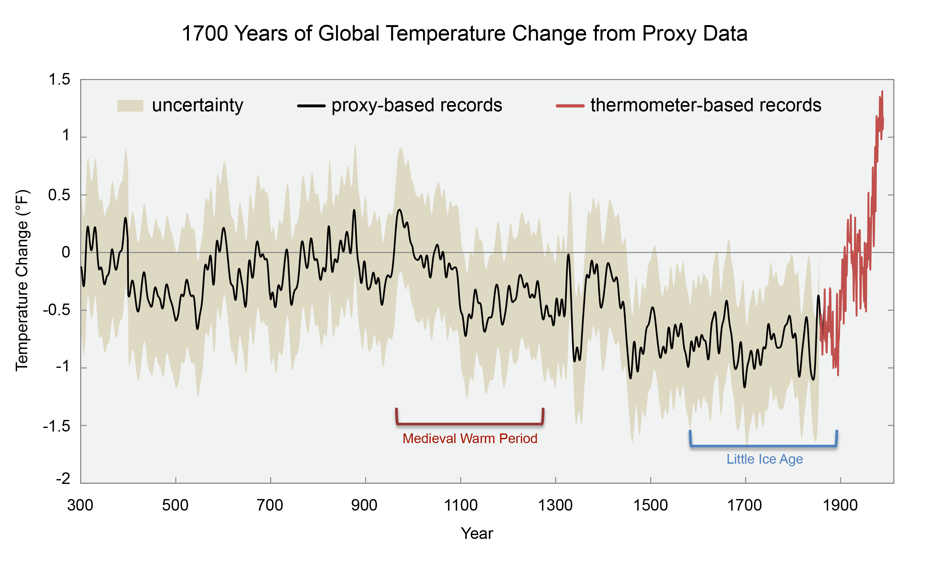
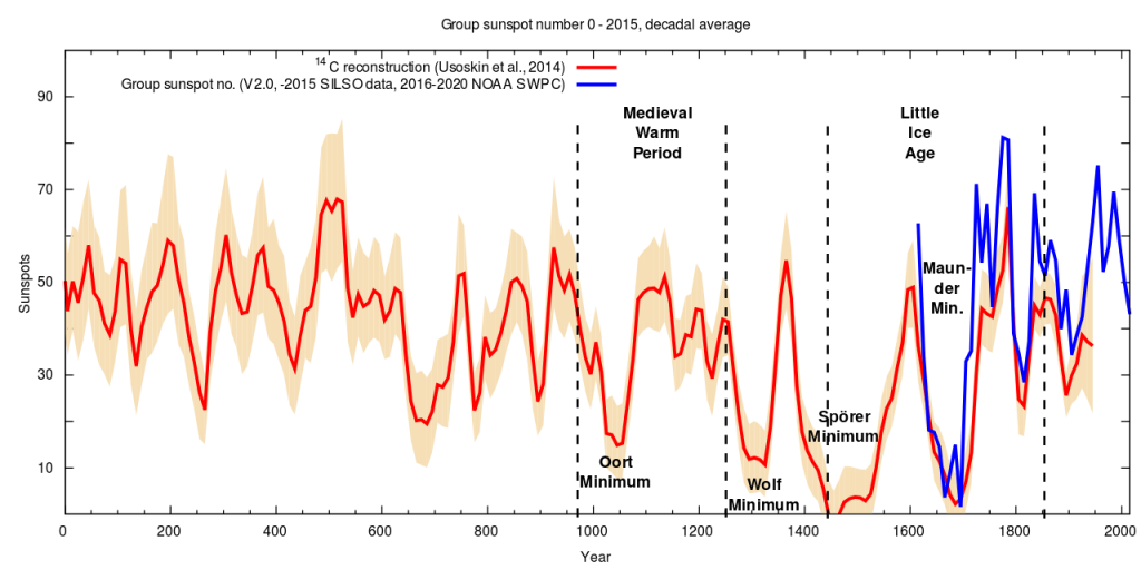
Most sources of data indicate that there was a distinct cold period that lasted from around 1450 to 1850 CE, known as the “little ice age“, although opinions differ on exactly when its start and end should be placed. European paintings from this era show bodies of water frozen over that have seldom frozen in the years since, while tree ring data show a succession of particularly cold intervals on the scale of decades. One of these coincides with a period, the “Maunder minimum”, in the late 1600s to early 1700s CE when astronomical observations record very few sunspots, and carbon-14 measurements imply that the solar wind was slightly less powerful, suggesting that the output of the Sun may have been reduced by perhaps a quarter of a percent. Earlier, similar-looking cold periods may have the same explanation.


Between these cold periods some warm intervals also appear. The “medieval warm period” from about 950 to 1250 CE was characterized, for example, by the raising of crops and farm animals in Iceland and southern Greenland, in areas where these activities became impractical after 1250 CE. Another wam period, the “Roman warm period” may have occurred between about 250 BCE to 400 CE.
For these proposed warm and cold intervals, the majority of historical proxy data come from the northern hemisphere. Some research involving the isotopic record in other parts of the world suggests that although these intervals were indeed globally slightly warmer and cooler, the timing of the warmest and coldest intervals varies in different parts of the Earth, so they may not be globally synchronous events.
Changes on the scale of years to decades
Exceptionally cold summers
Historical records over the last 250 years have recorded intervals with particularly cool summers characterized by poor harvests and widespread famine in parts of the world with temperate climates where food supplies are typically otherwise sufficient.
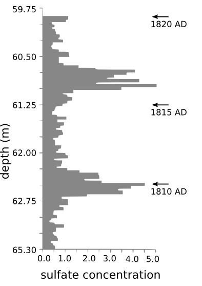
In 1816 CE, Europe experienced what was described as a “year without a summer” leading to widespread crop failures and famine. Similar effects were experienced in North America and in China. Global surface temperatures are estimated to have been depressed by about 0.5°C. The following two summers in 1817 and 1818 CE were also cooler than average.
These effects have been convincingly correlated with the eruption in April 1815 of the subduction-related arc volcano Tambora in what is now Indonesia, which was the largest volcanic eruption in historical records. The explosion put about 100 cubic kilometres of tephra into the atmosphere, and it is believed that the additional albedo and absorbtion of energy by the suspended ash affected climate for the following years.
Comparable global cooling effects occurred in the years following the eruptions of other large subduction-related volcanoes: Karakatau, also in Indonesia, in 1883, and Pinatubo in the Philippines in 1991.
El Niño Southern Oscillation (ENSO)
Other climate variations on the scale of years are apparent in records of weather when years are compared.
One such phenomenon is named “El Niño”. On the Pacific coast of S America, El Niño is observed in December of certain years. (The name means “newborn boy” and is derived from Christian festivities that occur at this time of year.)
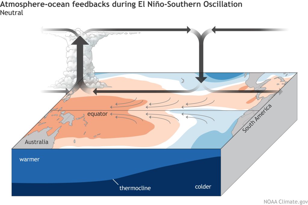
In years without El Niño conditions, air and water flow along the intertropical convergence zone in the Pacific is east-to-west and the most intense low pressure is in the W, near Australia. Nutrient-rich cold water rises to the surface along the coast of South America, driven by Ekman transport that moves water westward, increasing the fertility of fishing grounds along the South American coast.
In El Niño years the point of lowest pressure moves to the central Pacific. Wind and water flow along much of the ITCZ is then west-to-east. Upwelling of nutrient-rich water off South America is impeded, leading to poor fish catches.
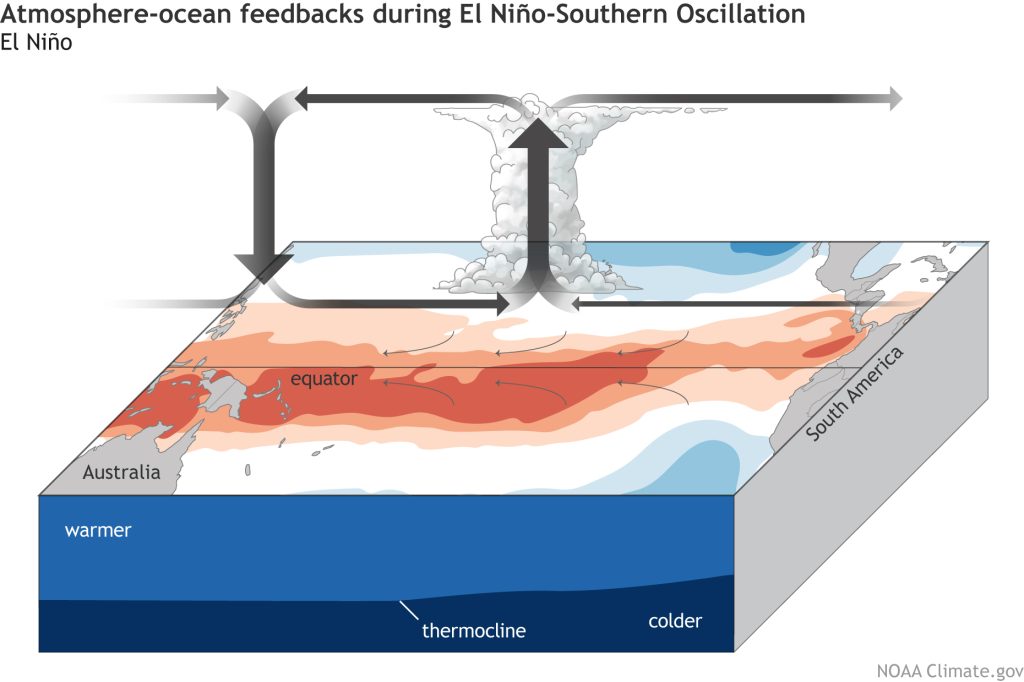
An opposite fluctuation, leading to unusually intense upwelling along the South American coast, is known as La Niña (newborn girl)
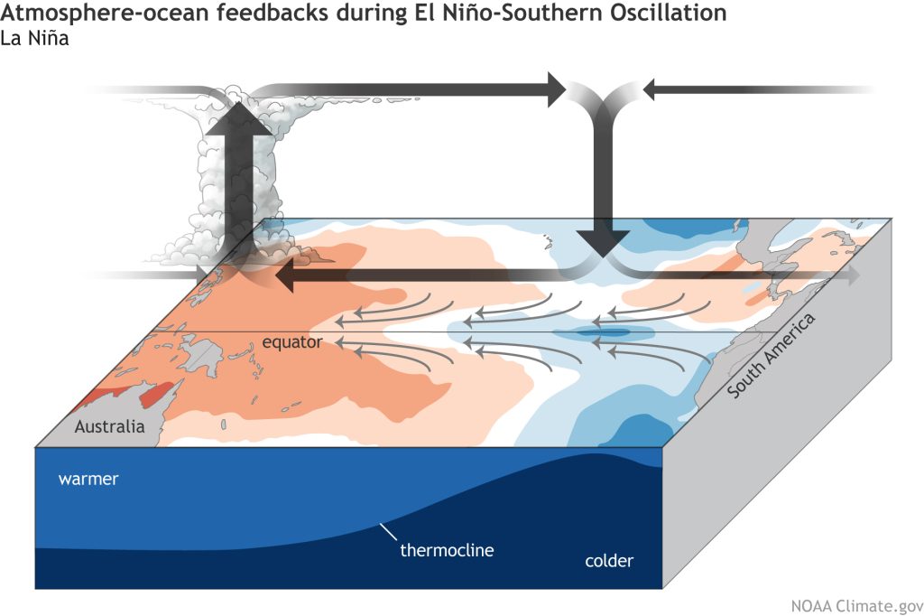
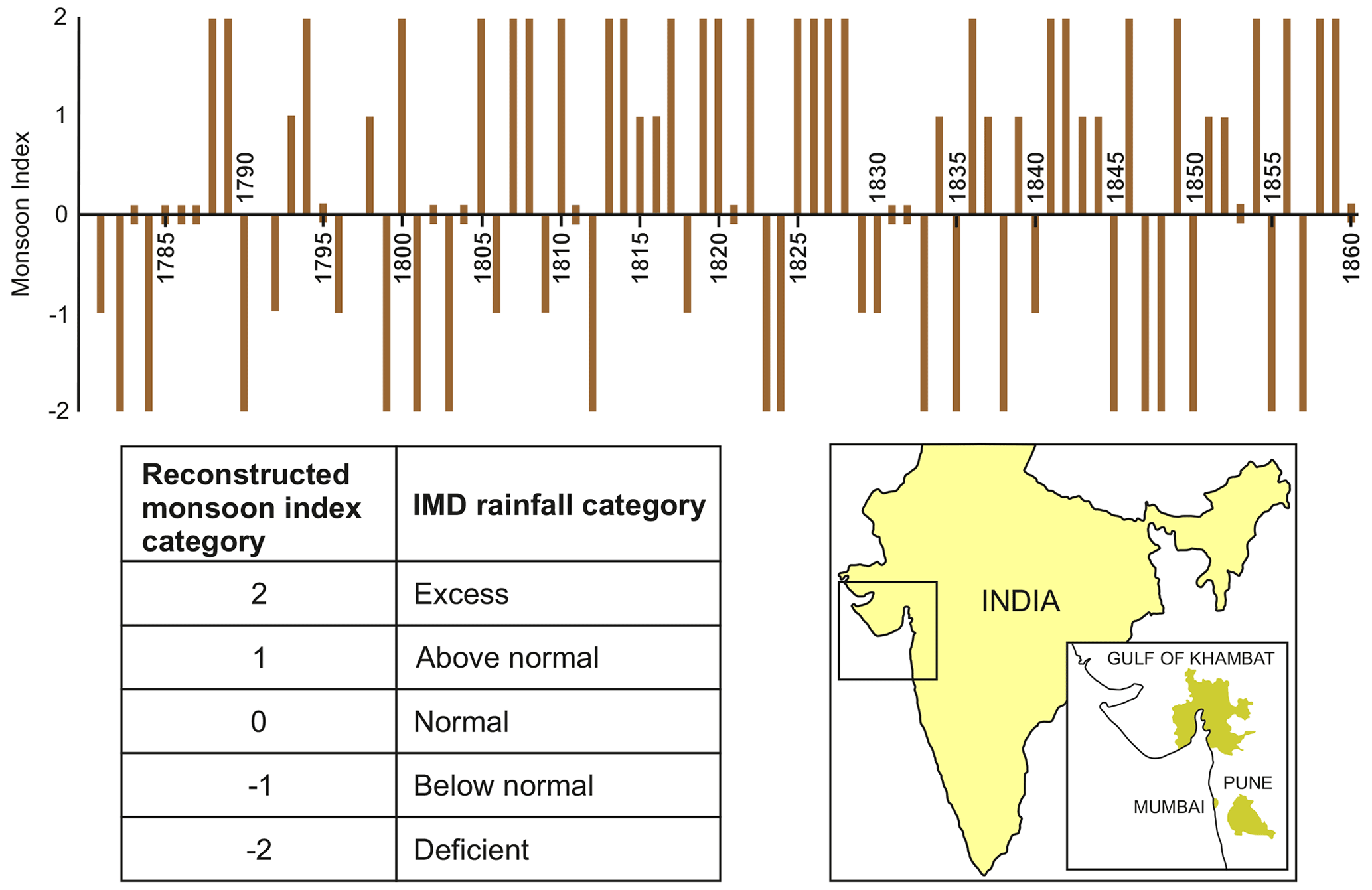
El Niño has been correlated with weather effects elsewhere in the world. For example, some oceans experience fewer tropical cyclones, while in others, the cyclones follow different paths in El Niño years. El Niño years have been shown to coincide with years in which the Asian monsoon is weaker, leading to drought conditions in parts of the Indian subcontinent.
The causes and effects of the El Niño Southern Oscillation are both poorly understood and are the subject of ongoing research, which is complicated by recent anthropogenic climate change, which has been modifying the atmosphere during the period when instrumentation and modelling techniques have begun to be capable of addressing these problems.
Anthropogenic change since 1700 CE
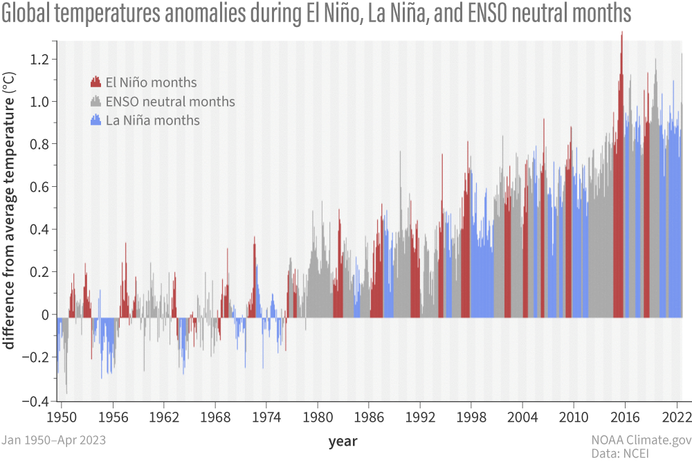
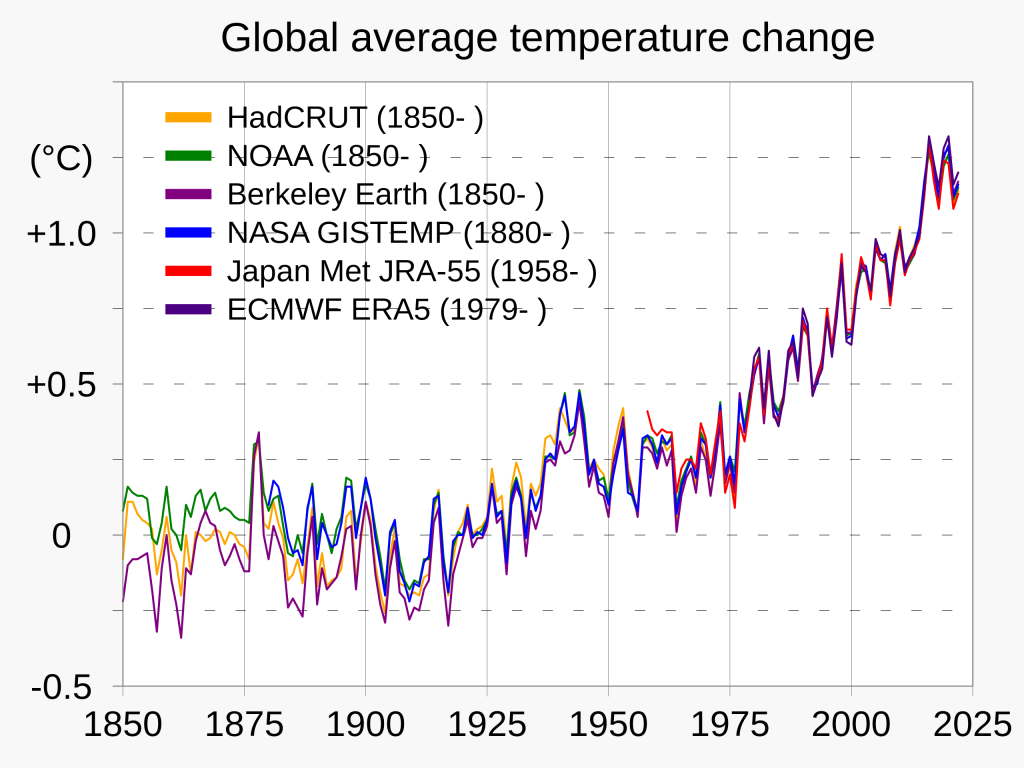
From about 1700 onwards, the Earth has seen an overall trend of rising surface temperatures, although this is punctuated by fluctuations associated with ENSO and cold pulses associated with volcanic events. Because of these sporadic cooling episodes, the reality of global warming was fiercely contested in the 1990s and early 2000s CE. However, the scientific records of this warming show an indisputable upward trend. During the period of direct instrumental measurement, the warming is shown in most records to be well over 1°C at the time of writing (2023), though the amount of warming varies from place to place on the Earth’s surface.
This warming trend has coincided with increasing delivery of carbon dioxide to the atmosphere as a result of human activites, mainly the burning of fossil fuels at a rate much greater than the return of reduced carbon to the Geosphere. This phenomenon has serious consequences at the surface of the Earth — loss of sea ice, rising sea-level, changing weather, increasing wildfire, ocean acidification, and others. The resulting controversies have led to a surge in research on climate change and the way it is driven, which we shall examine in the next section.
Forcings and feedbacks
Forcings
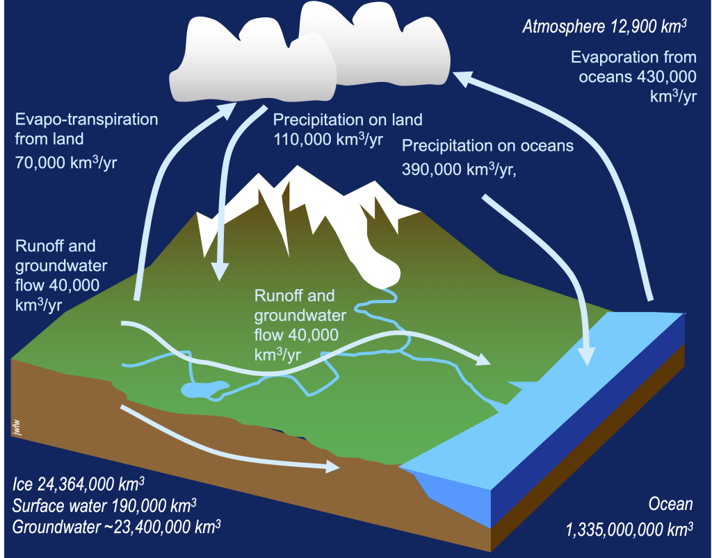
Earlier chapters on energy and on cycles mainly treated Earth systems as being in a steady state. That is to say, the fluxes (or energy, water, carbon etc.) in and out of each reservoir were equal, with the result that the sizes of the reservoirs didn’t change over time. For example, in the hydrologic cycle, the flow by evapotranspiration into the atmosphere (430,000 + 70,000 = 500,000 km3/yr) was shown as exactly in balance with the flow out of that reservoir by precipitation (110,000 + 390,000 = 500,000 km3/yr). Similarly, in the case of energy, the fluxes in and out of the Earth are shown as approximately balanced at 174,000 TW.
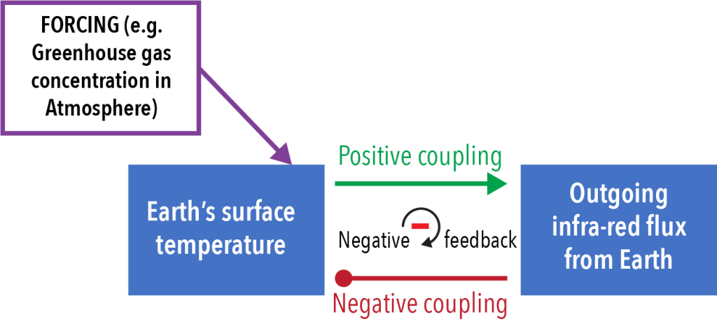
However, Earth systems are not always balanced in this way. If the fluxes in and out of a reservoir do not balance, the reservoir grows or shrinks over time. Factors that influence change of this type are known as forcings. [3] For example, the removal of hydrocarbons from the Geosphere and their release, after oxygenation, as carbon dioxide is an example of a forcing that changes the amounts of both carbon dioxide and heat in the atmosphere over time. The term forcing is most often used to describe changes in the energy cycle but in principle a forcing can apply to any external effect that modifies the fluxes in any cycle over time.
Forcings that operate on a system can originate within the system itself, or they can come from outside. Within the climate system we can recognize:
External forcings (examples): originate outside the climate system:
- Tectonic events
- Orbital changes
- Solar energy changes
- Volcanic activity
- Anthropogenic changes
Internal forcings (examples): originate within the climate system:
- Greenhouse gases
- Aerosols
- Albedo changes
- Oceanic and atmospheric circulation patterns
As we shall see, depending on the scale of the system being examined, some internal forcings may also be regarded as feedbacks.
Feedbacks
If a forcing were to operate over a long period of time without hindrance, the fluxes and reservoirs it influenced would continue to change, becoming larger or smaller indefinitely, without control. In practice, most forcings to not operate in isolation. Typically, a forcing will change conditions in the system, such that the forcing is either inhibited or enhanced. The processes that cause a forcing to be changed in response to its own effects are known as feedbacks. We recognize two types of feedback:
- Negative feedback: a process in a cycle changes conditions in such a way that the original process is inhibited.
- Positive feedback: a process in a cycle changes conditions in such a way that the original process is enhanced.
Negative feedbacks
To analyse feedbacks and forcings, it’s helpful to construct flow diagrams that show how one phenomenon influcences another. The influences are called linkages. In the following sections[4], positive linkages, where an increase in one phenomenon causes an increase in another, are shown by pointed green arrows.
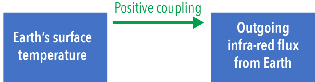 This diagram says that an increase in Earth’s surface temperature leads to an increase in the heat radiated from the Earth, a phenomenon shown by all objects.
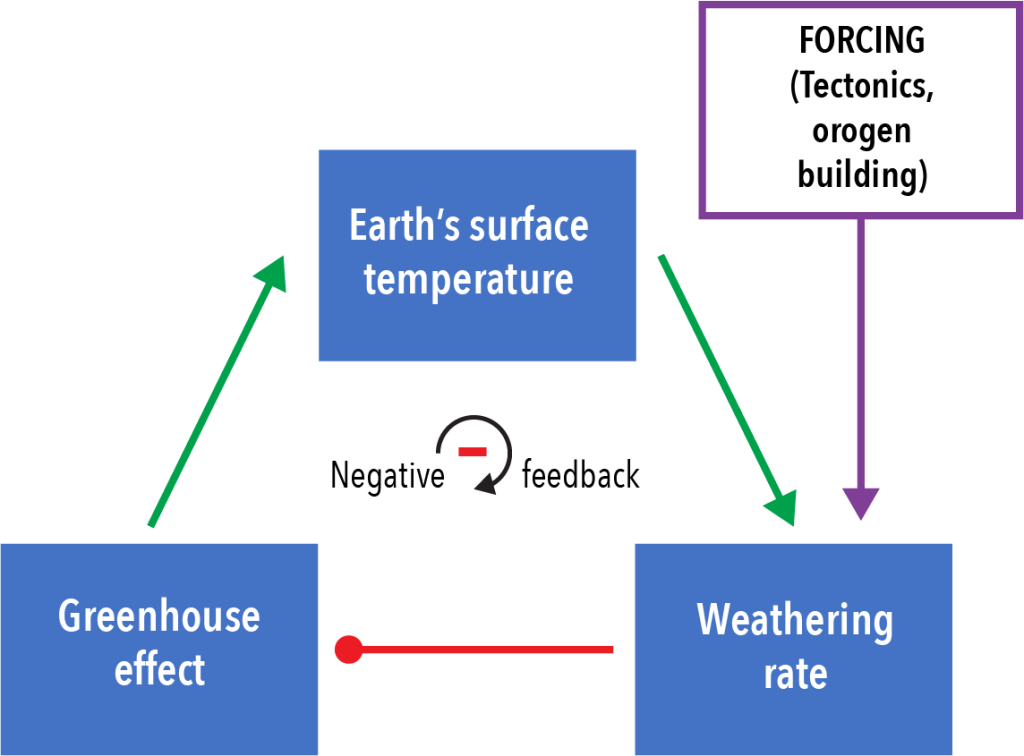
On the other hand, when an increase in one phenomenon leads to a decrease in another, the two are linked by a line with a circular end, shown in maroon. In this case we indicate that an increase in the loss off heat causes a decrease in the Earth’s surface temperature.
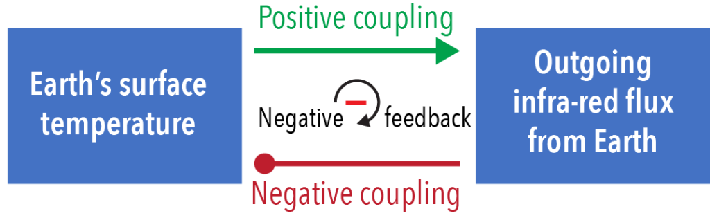 These two linkages are joined in a simple feedback loop. Because this feedback loop contains one negative linkage, we describe the loop as negative feedback. If an increase in Earth’s surface temperature occurs as a result of an external forcing, the Earth will respond so as to reduce the effect of that forcing.
In practice there are at least three processes in play within the Earth that support this negative feedback
- Planck or black-body feedback. If the top of the troposphere is warmer, more energy is radiated into space
- Cloud-albedo feedback: Warmer oceans evaporate more water, increasing the amount of cloud. Cloud is white and reflects more solar energy into space.
- Lapse-rate feedback: the adiabatic lapse rate of condensing air is lower, so more heat is transported to the top of the troposphere when clouds are forming.
Positive feedbacks
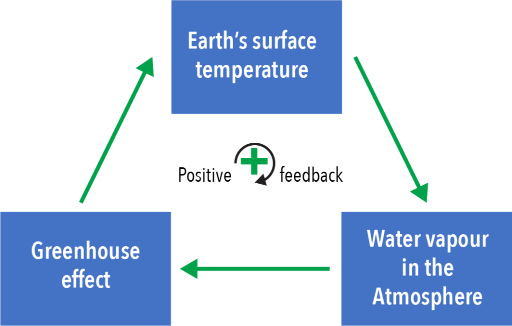
Unfortunately, this is not the only feedback in play. Changes in the Earth’s surface temperature also result in positive feedbacks.
First, increase in surface temperature puts water vapour into the atmosphere, and any water vapour that does not condense to form clouds acts as a greenhouse gas, absorbing the Earth’s outgoing infra-red radiation and sending some of it back to the surface. Hence warming the surface increases the greenhouse effect and leads to further warming, at least until saturation vapour pressure is reached.
Secondly, directly leads to the loss of ice cover — both land and sea ice — which reduces Earth’s overall albedo, and therefore leads to increased absorbtion of solar radiation and more increase in temperature. This positive feedback loop potentially can continue until little ice remains. It probably has a major role to play in the oscillation between glacial and interglacial conditions during icehouse conditions.
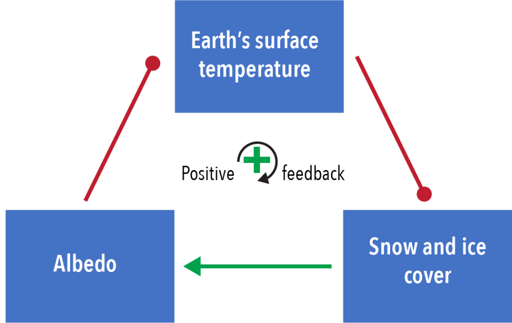
Notice that feedback loops containing no negative linkages, or containing an even number of negative linkages, are positive. Feedback loops containing one negative linkage (or any odd number) are negative.
Fast and slow feedbacks
The feedbacks described above operate rapidly: almost instantaneously in comparison with geologic time. They are known as fast feedbacks. However, there are other more complex feedbacks that come into play much more slowly after a forcing. For example, a rise in temperature may lead to changes in the biosphere that lead to the production of more or less greenhouse gas.
- Expansion or contraction of the most productive biomes
- Adaptations by plants that adjust their ability to capture carbon dioxide (e.g. changes in the number of stomata on plant leaves).
- Evolution of new species that take advantage of changed conditions
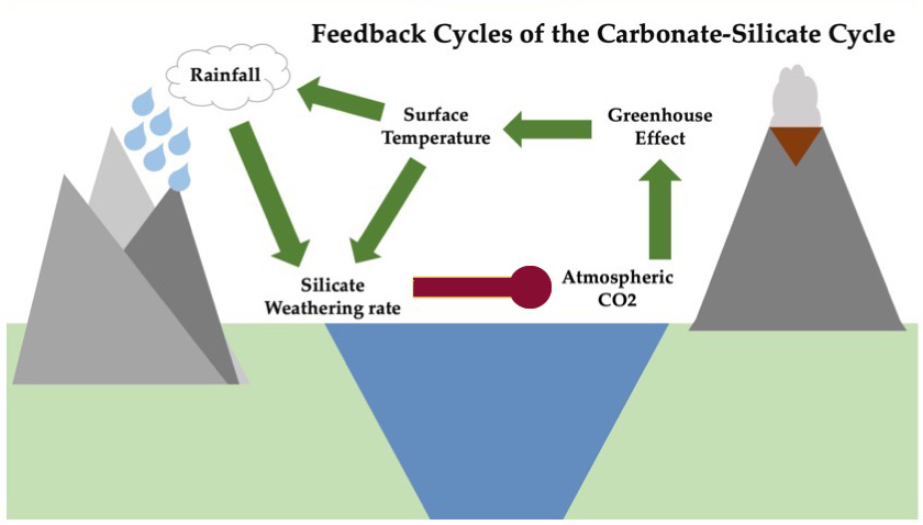
Another more complex slow feedback has involved the rock cycle. Increased temperature, and increased humidity, tend to increase the rate of chemical weathering. Because chemical weathering involves carbon dioxide, increased chemical weathering of silicate rocks leads to net removal of carbon dioxide from the atmosphere. Ultimately this carbon dioxide ends up in carbonate ions which are incorporated in carbonate rocks like limestone, causing a negative feedback that helps to moderate temperature increases and atmospheric carbon dioxide.
A simplified overall chemical equation for this process is
CaSiO3 + CO2 = CaSiO3 + SiO2
Calcium silicate + carbon dioxide = calcium carbonate + silica in solution
The carbonate is stored in the Geosphere until the carbonate rocks are either metamorphosed or partially melted, which may release the oxidized carbon back to the atmosphere as carbon dioxide. This cycle is known as the carbonate–silicate weathering cycle.
Positive feedbacks, if unchecked, can lead to runaway feedback, where the system moves unabated to an extreme condition. Runaway feedback may have played a role in:
- The development of snowball Earth conditions during the Proterozoic Eon, when the ice–albedo feedback loop continued until almost the entire Earth was covered by ice.
- The development of permanent greenhouse conditions beneath the carbon-dioxide-rich atmosphere of the planet Venus, allowing surface temperatures to rise above 450°C despite solar energy input only about twice that of Earth.
Fortunately, for most of Earth history it appears that negative feedbacks have offset positive feedback loops so that runaway feedback has not occurred.
Forcing and feedback
Despite the contrasting definitions of forcings and feedbacks, the distinction between the two is not always clearcut. This is because Earth systems are open systems, and what is chosen as a system is a matter of convenience. So, for an oceanographer investigating the oceans as a system, the addition of carbon dioxide from the atmosphere is a forcing that originates outside the system, and pushes the oceans towards lower pH. However, for a climate scientist studying the carbonate–silicate weathering cycle, that involves both the hydrosphere and the atmosphere, the solution of carbon dioxide in the oceans is part of a larger feedback loop. The distinction between forcings and feedbacks is therefore dependent on the choice of system under examination.
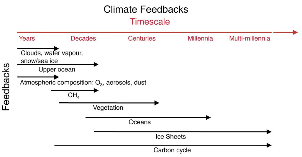
An additional complication in the analysis of feedbacks is the time dimension. Some feedbacks operate on a very short timescale. For example, when warming causes the melting of sea ice, the effect on albedo is apparent within a year. On the other hand, effects of warming on biomes, and particularly the colonization of new areas by plant species that are heat-tolerant or that can exploit rising carbon dioxide concentrations, may take decades or even centuries to come about. These factors may add a delay to the Earth’s feedback response to a new forcing.
Natural forcing and its effects
Tectonic forcing
The tectonic system generates forcings on several parts of the climate cycle:
- Major volcanic episodes deliver CO2 to the atmosphere. It has been suggested, particularly, that the development of large igneous provinces within continents has on some occasions produced exceptional amounts of CO2, leading to episodes of global warming.
- Plate movement alters the distribution of continents and oceans and thus the distribution of surfaces with different heat capacities, different biomes, and different albedo. The movement of Antarctica over the South Pole, following the breakup of Pangea, may have allowed the Antarctic Ice Sheet to start developing.
- Global thermohaline circulation is very dependent on the shape of the ocean floor. At the present day, North Atlantic deep water is able to escape from the Arctic Ocean and spread southwards, contributing to the “conveyer belt” that transports heat around the Earth as described in the section on ocean currents.
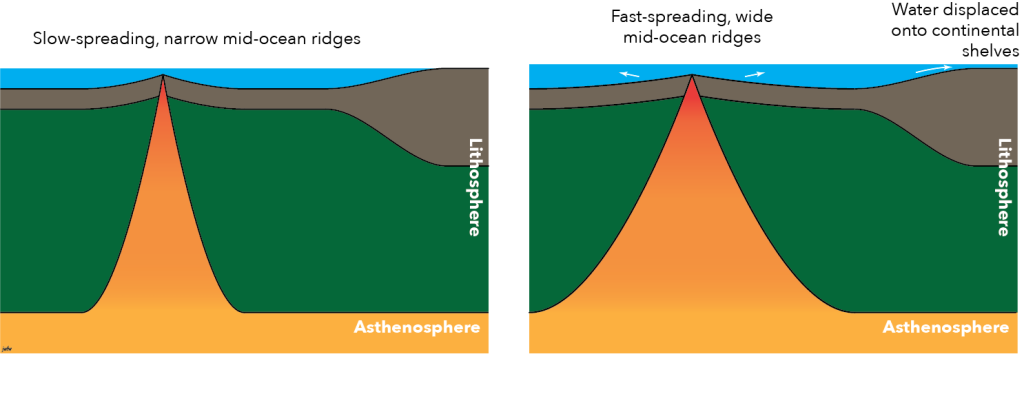
- It is likely that the total amount of mid-ocean ridge has varied as plates of the Lithospere changed configuration over geologic time. Mid-ocean ridges are sites of sea-floor volcanic activity, releasing carbon dioxide into the atmosphere, so increased sea-floor spreading has been associated with warming due to the greenhouse effect. However, faster sea-floor spreading makes larger mid-ocean ridges that displace water onto the continents forming wide continental shelves. The shallow, sunlit waters of continental shelves are one of the most organically productive parts of the hydrosphere and therefore tend to capture carbon dioxide, converting it to organic carbon. This acts to reduce the greenhouse gas impact of carbon dioxide released at the mid-ocean ridges. The last part of the Mesozoic Era, from ~100 to 66 Ma, were characterized by particularly broad continental shelves on which characteristic chalk sediment was deposited. This was a period of warm greenhouse conditions, suggesting that the greenhouse effect of carbon dioxide released from the mid-ocean ridges exceeded the ability of the wide continental shelves to absorb it.
-
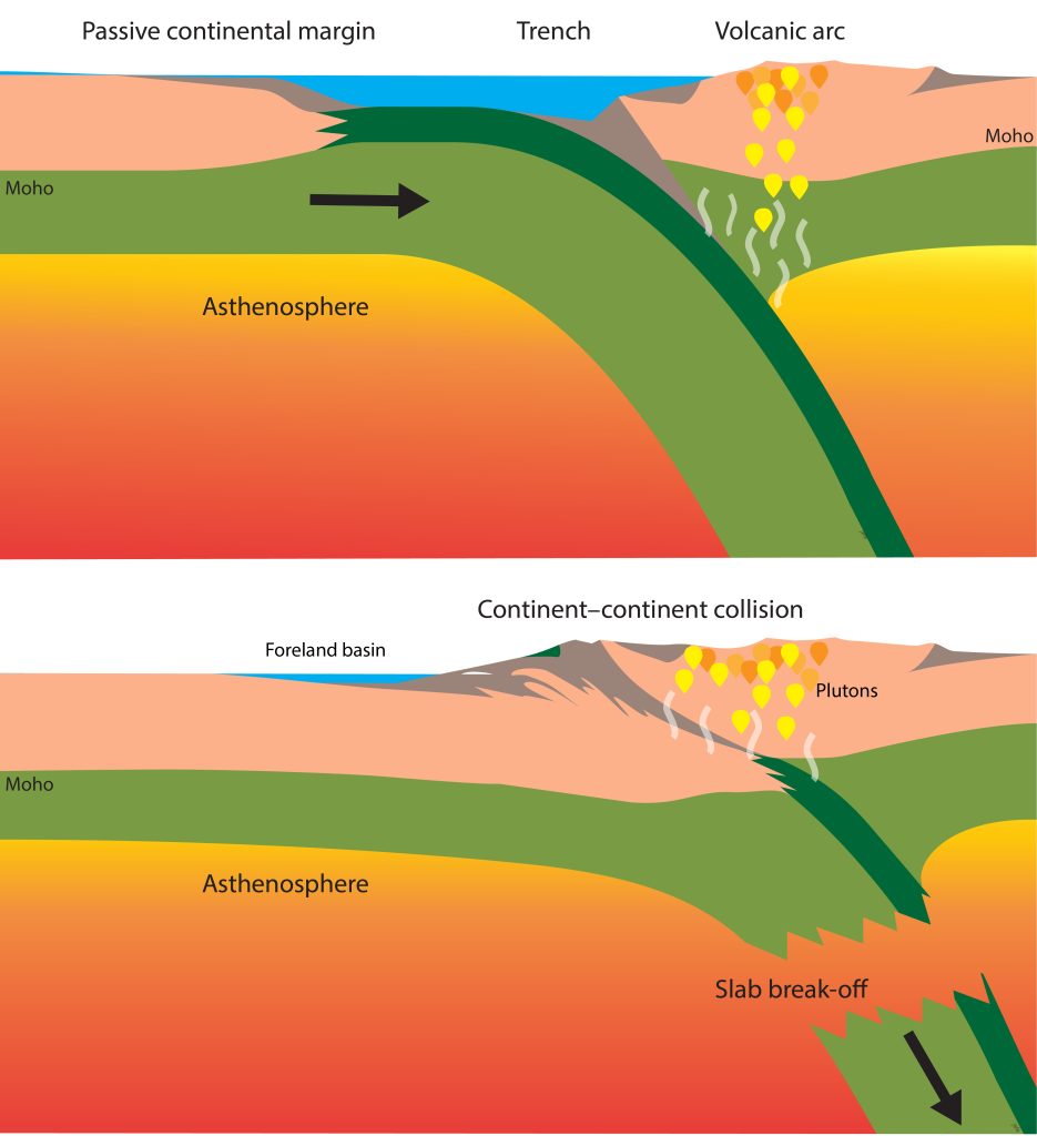
Tectonic processes such as orogenesis by continent-continent collision may have produced major purturbations to the climate system, potentially leading to icehouse conditions. JWF Waldron CC BY-SA Orogenesis, or mountain building, affects global and regional climate patterns in a number of ways. Mountains cause orographic lifting, prompting heavy rainfall, including monsoon rainfall, on their windward sides. On their leeward sides, rain shadow areas may contain dry deserts. On a global scale, mountain building increases global weathering rates, leading to more activity in the carbonate-silicate weathering cycle, which acts to reduce the amount of carbon dioxide in the Atmosphere. This is especially true of mountain ranges in warm humid environments and those impacted by monsoon rains. Major orogenic episodes in equatorial latitudes are therefore predicted to reduce the amount of carbon dioxide in the Atmosphere and cool the Earth. The onset of Cenozoic icehouse conditions approximately coincided with the collision of India with Asia at about 50 Ma, which eventually led to the building of the Himalaya. This tectonic event may have been a major climate forcing, that led to steady global cooling since 50 Ma.

Solar forcing
Long-term Solar forcing
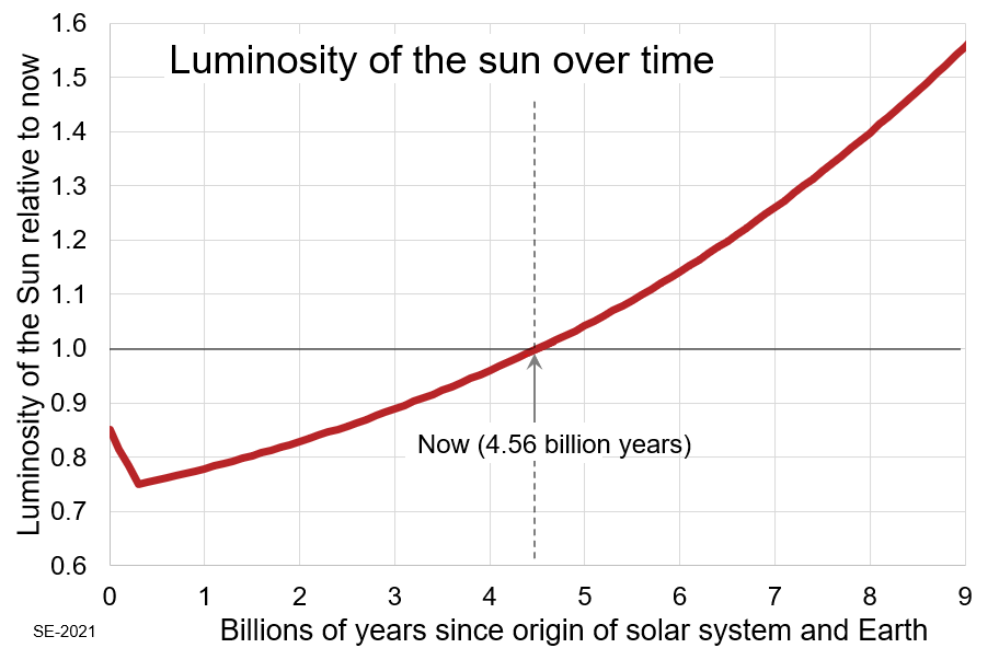
Changes in the energy output of the Sun are also forcings that affect climate. On the longest time scale, modelling of the nuclear fusion processes that fuel the Sun, combined with astronomical observations of similar stars at various stages in their life history, suggest that the Sun’s output has steadily increased since the origin of the Solar System at ~4.6 Ga. This would be predicted to have caused steady global warming as a direct result.
However, over the same period of time, the rise of photosynthesis in the biosphere has reduced the amount of carbon dioxide in the atmosphere. Because carbon dioxide is a greenhouse gas, this is predicted to have lead to steady global cooling. Additional cooling may have been forced by a reduction in geothermal energy resulting both from the overall cooling of the Earth and from the reduction in the amount of energy from radioactive decay, because of the half-lives of radioactive elements.
The actual climatic history in the Proterozoic Eon probably reflects the interaction between these forcings. When warming due to increased solar output was the dominant influence, greenhouse conditions persisted. However, when the biosphere caused a rapid reduction in carbon dioxide, cooling resulted in the formation of ice-caps, and then the ice–albedo positive feedback took over, cooling the Earth in until much of the surface was covered with ice, ther snowball Earth condition.
Glacial conditions would have reduced biological activity to a minimum, so during snowball Earth, the rate of photosynthesis would have declined, a negative feedback. Meanwhile, carbon dioxide release from volcanic activity at plate boundaries would have continued. Because of the lack of photosynthesis, carbon dioxide could accumulate in the atmosphere unchecked. The greenhouse effect would eventually have led to melting of the ice cover in some places. The reduced albedo would take effect immediately, whereas the biosphere would take time to recover its photosynthesizing capability, so warming would have been rapid, returning Earth to a greenhouse condition.
Short-term Solar forcing
Variations of Solar irradiance on the scale of years to decades are relatively well known, and in recent years it has been possible to measure solar output directly.
Solar output rises and falls in step with the sunspot cycle, an 11-year rise and fall in the number of sunspots — small, less bright patches on the face of the Sun that are associated with major magnetic storms and output of particles that form the solar wind. Periods of high sunspot activity are associated with higher irradiance, but the effect is small: around 1 W/m2 on a total irradiance of ~1366 W/m2 or less than 0.1%.
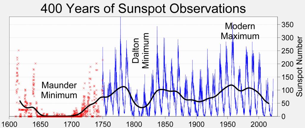
Some slightly longer term effects are also known. Systematic sunspot records go back to around 1600 CE, and a period from ~1650 to ~1715, known as the Maunder minimum, was characterized by very low sunspot numbers. We also know that at that time the solar wind was less intense; this has been determined by comparing carbon-14 dates (dependent on the formation of carbon-14 by the action of Solar wind) with dates derived from varve and tree-ring counting. From this it is known that the Maunder minimum also coincided with a decline in the strength of the solar wind and it has been suggested that this may have corresponded to a decrease in irradiance by as much as 0.25%. Earlier carbon-14 data indicate that other minima occurred during the time of the little ice age. A 0.25% drop in irradiance is not sufficient, on its own, to account for these climate fluctuations, but when combined with amplification by positive feedbacks like the ice–albedo feedback it is the best explanation for natural climate changes on a scale of decades like the Maunder mimimum.
Orbital forcing
Cycles that occur naturally in the Earth’s orbit are known as Milankovitch cycles after their discoverer. They are described in detail in the section on the Earth’s orbit in the Solar System.
Movie illustrating variations in eccentricity. Credit: NASA/JPL-Caltech. Public domain. https://climate.nasa.gov/system/video_items/143_eccentricity_with_border.m4v
Three main periodicities are known:
- Changes in the eccentricity of the Earth’s orbit, with periods of about 100,000 years and 400,000 years;
- Changes in the obliquity (or tilt) of the Earth’s axis relative to the plane of its orbit, with periods around 41,000 years; and
- Changes in the position of the solstices and equinoxes relative to the elliptical orbit, with periods around 23,000 years, known a the precession of the equinoxes.
The other two cycles don’t affect the total irradiance but they do affect the distribution of energy between the poles and the equator, and between the northern and southern hemisphere. Both can have effects on climate, because in the present-day tectonic system, continental areas are mainly concentrated in the northern hemisphere. However, the North Pole itself is located in the Arctic Ocean whereas the South Pole is in the continent Antarctica.
As a result, although the changes to the total Solar irradiance are less than 1%, the changes in irradiance resulting from Milankovitch cycles are much larger — up to 13% — at a latitude of 65°N, where the maximum amount of land is located. Because heat is only slowly redistributed to and from continental interiors, Milankovitch forcings, combined with positive feedbacks, are sufficient to trigger the oscillation of the Earth’s climate between glacial and interglacial intervals that can be observed in proxy data for the last 2.6 Ma.
The match between the predicted effects of Milankovitch cycles and climate proxies from Antarctic ice cores is good. There is little doubt, therefore, that the glacial/interglacial cycles tthat occurred during both the late Paleozoic and late Cenozoic icehouse intervals have been driven by orbital cycles.
One notable aspect of the proxy data is that temperature and atmospheric carbon dioxide are correlated throughout the ice-core record, so there is clearly a positive feedback operating between the two. However, it’s clear that the primary forcing (before anthropogenic effects came into play) was Milankovitch orbital cyclicity. How then, does the interplay of climate and temperature work? A possible answer involves a close examination of the temperature and carbon-dioxide curves in the transition from the glacial maximum to interglacial periods.
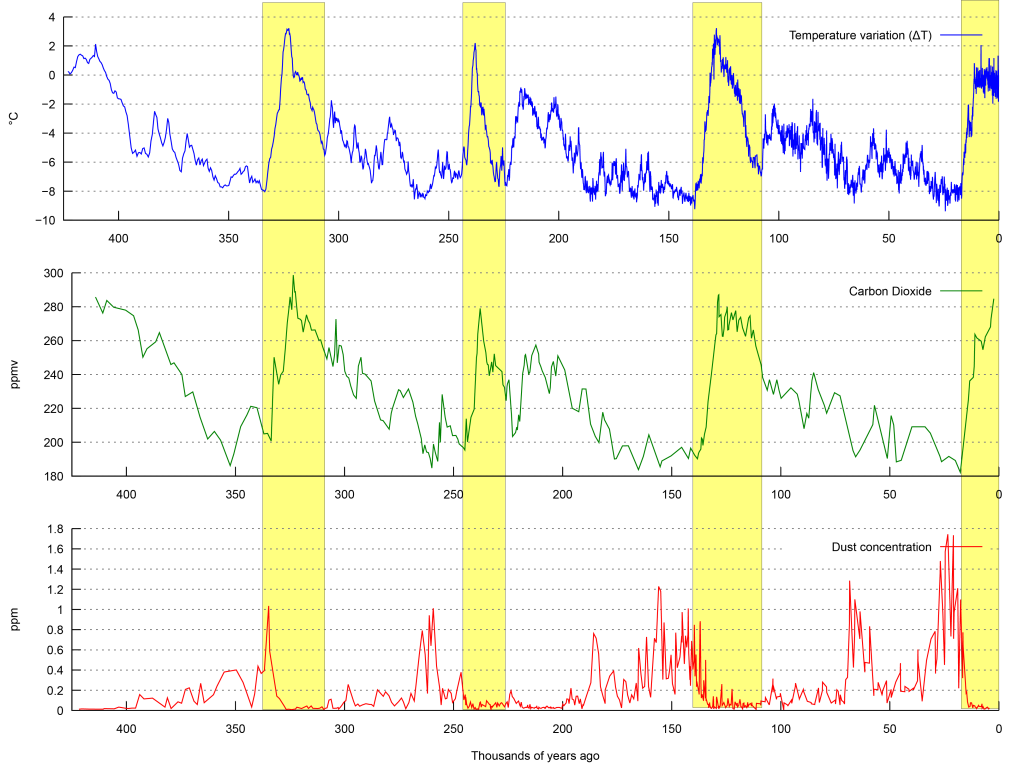
The first effect seen is a rise in temperature. Subsequently, there is a rise in carbon dioxide, probably caused by exposure of permafrost and other carbon stores, exposed by receding ice. The rising carbon dioxide curve eventually overtakes the temperature curve, showing that the initial small effect of Milakovitch forcing was amplified by a positive feedback resulting from the greenhouse effect of carbon dioxide. It is notable that global warming in the last 300 years has not followed this pattern. Industrial release of carbon dioxide preceded warming during human industrial activity.
Anthropogenic climate change
Anthropogenic additions to the atmosphere
What happens when a new forcing is added to the climate system? Changes induced by humans are described as anthropogenic from two Greek words meaning “human” and “formed”. Like the Latin word homo, the Greek anthropos referred to any human regardless of gender. Some writings in English use “man” in this way, referring to anthropogenic changes as “man made”. We avoid this usage because in English the word “man” can also be used to refer specifically to a male human, a usage that has led to serious ambiguity in some scientific writing.
Carbon dioxide
Since the industrial revolution between about 1760 and 1840 CE, humans have released about 375 Gt of extra carbon as carbon dioxide into the Earth’s atmosphere. The current (2023) rate of release is about 10 Gt per year and, despite rising concern, continues to increase.
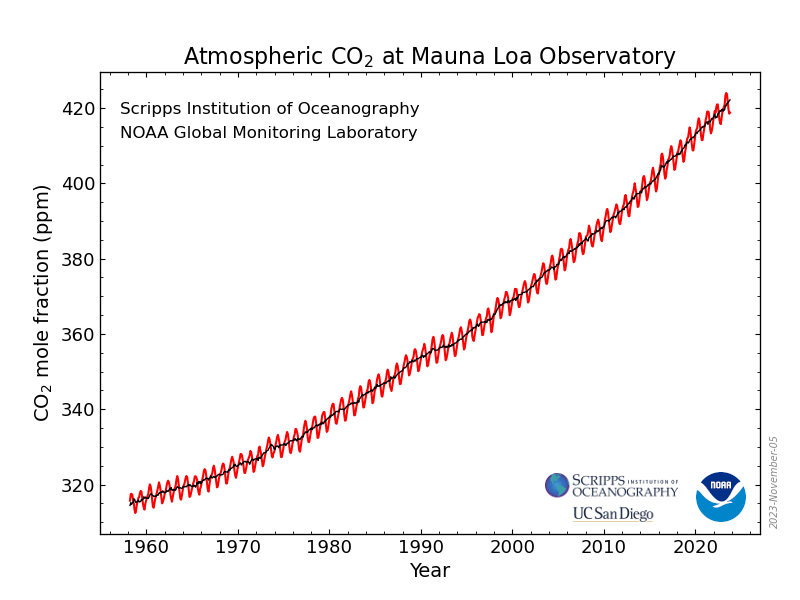
Only around half of this carbon dioxide still resides in the atmosphere. The remainder has been about equally split between the oceans (where it is mainly present as bicarbonate ions HCO3–) and the biosphere (where it has been stored as organic carbon). These two processes represent negative feedbacks that to some extent offset the greenhouse warming effect of anthropogenic carbon dioxide, although they respond more slowly than positive feedbacks like the ice–albedo feedback. However, solution of carbon dioxide in the oceans is a problem in itself, as it leads to acidification which has detrimental effects on organisms, especially those, like corals, that extract calcium carbonate from seawater to build skeletons.
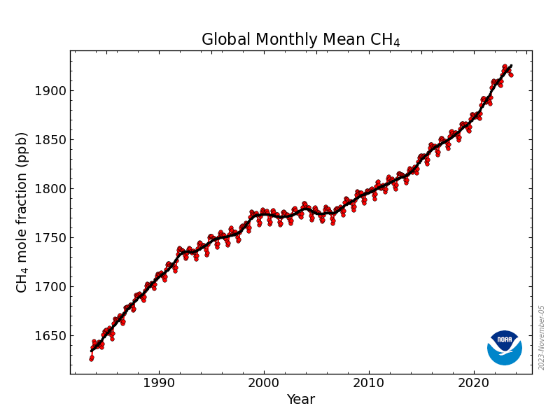
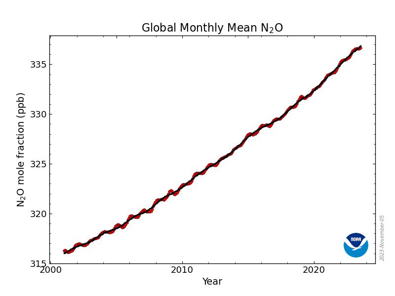
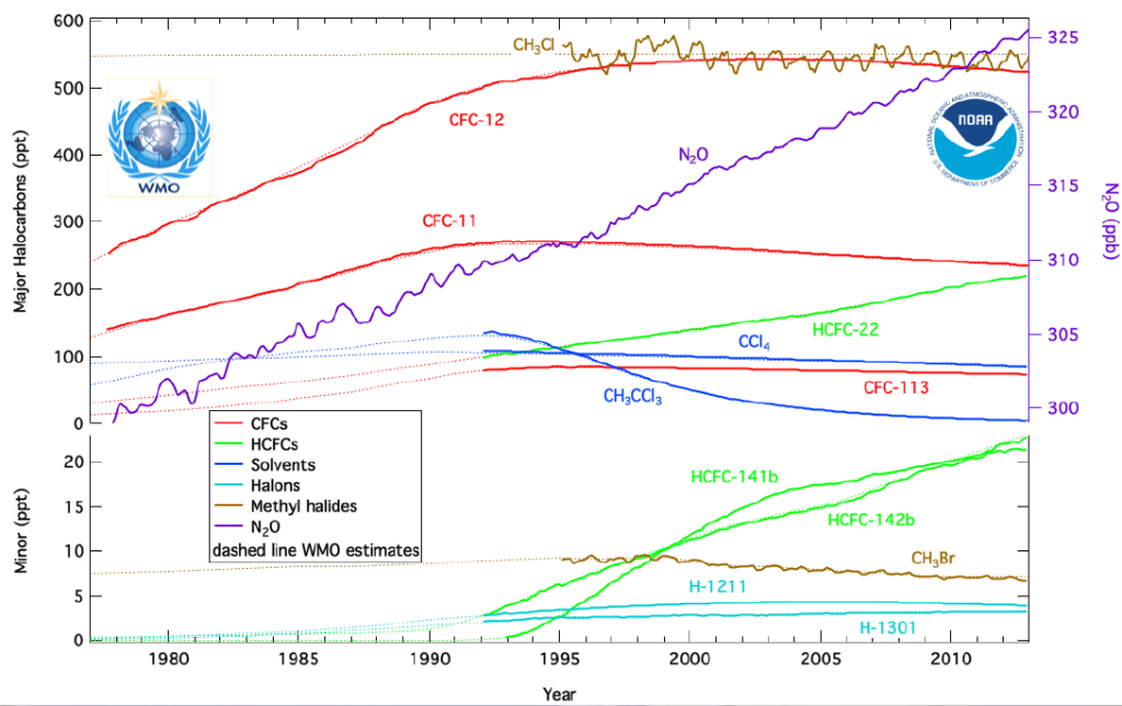
Other greenhouse gases
Other greenhouse gases contributed by humans include methane (CH4), nitrous oxide N2O, and a category of gases known as flourinated gases, including chloro-fluoro-carbons (CFCs) that are widely used in refrigeration systems. In general, the output of all these gases has increased over time. However, CFCs also have destructive effects on Earth’s ozone layer, at the top of the stratosphere. Global concern over this effect led to international agreements to limit their use, which has successfully reduced emissions of some of these gases since about 2000 CE.
<
Effects of anthropogenic gas
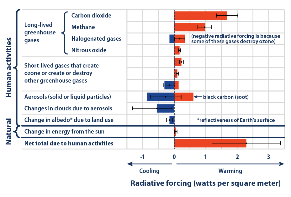
Radiative forcing
The effects of greenhouse gases are typically evaluated in terms of radiative forcing. That is to say, the imbalance between solar irradiance(in watts per square metre) and output long wavelength radiation that results from the additional of greenhouse gas[5]. Radiative forcing is therefore a measure of the rate at which the amount of heat stored in the atmosphere changes as a result of the presence of added greenhouse gas.
- Radiative forcing due to carbon dioxide[6] is currently ~2.2 W/m2, out of a total irradiance of 1366 W/m2.
- If all the other greenhouse gases are included, this figure rises to 2.7 W/m2.
Although this amount sounds small — it amounts to just under a quarter of a percent of solar irradiance — it is comparable in magnitude to the orbital and solar forcings that have caused major climate change in the past. The reason a small change in energy input is able to make a large difference to climate is because several feedbacks respond to radiative forcing, and the positive feedbacks are more effective than the negative feedbacks.
Temperature changes
Turning changes in radiative forcing into changes in temperature is not straightforward, becasue of the range of feedbacks involved, all of which operate on different time scales.
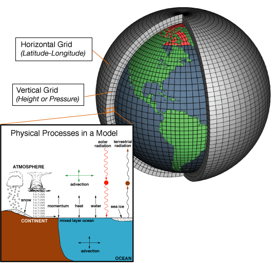
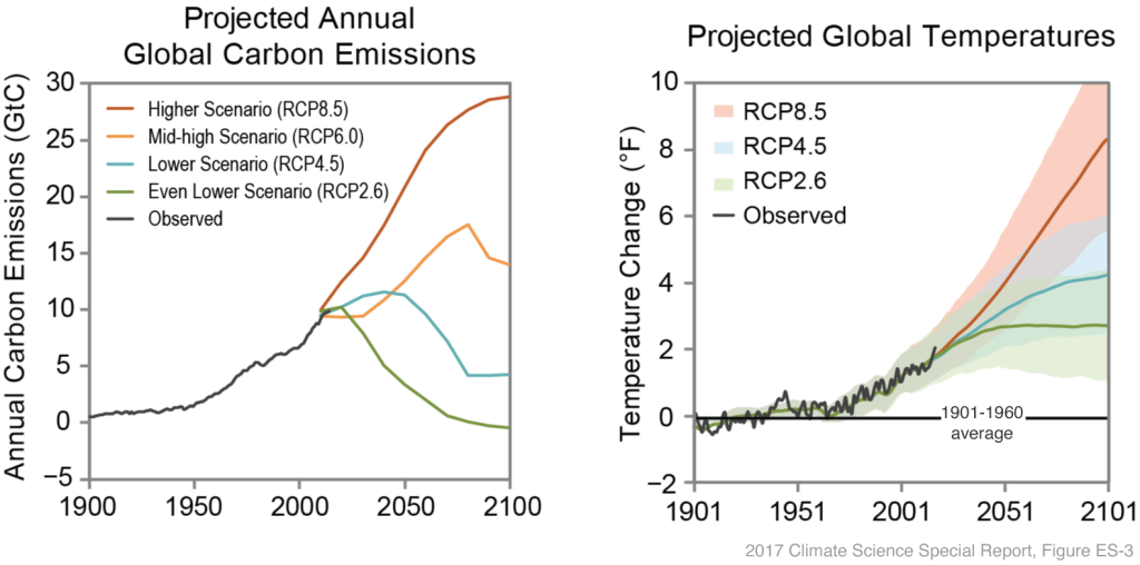
Typically, computer climate models known as general circulation models (GCMs), or global climate models , are needed in order to evaluate the effects of different forcings on the climate system. Any computer model is effectively a hypothesis about how the Earth system works, which should be tested. However, if we wait around for a prediction to come true (or not) it will be less useful, so a common strategy in computer modelling is known as hindcasting. In hindcasting, a historic set of data (perhaps from 10 or 50 years ago) is used as input to the climate model, and the model is used to predict events going forwards from that point. The predictions can be compared with present-day data in order to test the model.
As a result of these efforts it’s possible to show that in the long term (on a scale of centuries) the radiative forcing effect of a doubling of Earth’s atmospheric carbon dioxide from its pre-industrial value of 280 ppm to 560 ppm would be a global temperature rise of about 1.2°C on average. Once feedbacks are taken into account, that value rises to 3°C.
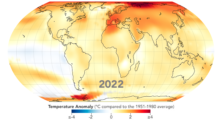
The effects of warming are not evenly distributed. Because of the very large roles of Arctic sea-ice melting and permafrost breakdown, in northern land areas in positive feedback loops, the predicted warming in the Canadian arctic is approximately double the global average, a phenomenon known as Arctic amplification. Some areas of the Canadian Arctic have already seen warming by as much as 4°C.
Effects on ice
A first and obvious effect of rising temperature on the Hydrosphere is the loss of ice: sea ice, land glaciers, and permafrost.
The melting of Arctic sea ice is documented from satellite observations, and is a major positive feedback in the climate system, because sea ice has a very high albedo, and the open water that remains after melting is very dark. Loss of sea ice impacts marine mammals such as polar bears and seals that spend part of their life cycle on floating ice.
Loss of land ice is apparent in many alpine glaciers, in which ice is melting in the zone of ablation at a rate faster than it is supplied at higher elevations in the zone of accumulation
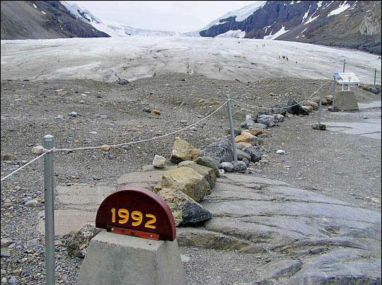
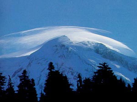
Despite the overall trend of glacier retreat, there are a few glaciers that are advancing. This can occur, even during periods of global warming, if a glacier is close to warm seas that deliver a large amount of water vapour to the atmosphere. Onshore winds may undergo orographic lifting, to produce increased amounts of snow in a glacier’s zone of accumulation. In exceptional cases this is enough to offset the increased melting that the glacier incurs due to warming temperatures.
The largest loss of ice in the present-day world is occurring in the Greenland ice sheet. Significant ice loss is also occurring in Antarctica, especially from ice shelves (effectively floating glaciers) that form where the ice sheet spills onto the southern ocean.
A third region of ice loss is partially hidden from view: melting of permafrost is a major concern in northern communities of Canada, where community infrastructure built on permafrost is subject to sudden and unexpected mobilization of frozen ground. Permafrost also traps organic carbon and prevents it from being oxidized by microbes and converted to carbon dioxide. Melting of permafrost allows this conversion to take place, providing a positive feedback that accelerates warming.
Effects on oceans
Sea-level change
Global warming affects sea level in at least two ways. First, water expands as it is heated, and second, melting of ice on land adds water to the oceans. (Note that melting of floating ice does not affect sea level, because floating ice displaces its own weight of water.)
To measure sealevel change, it’s necessary to make measurements over a period of time, to average out the effects of waves (seconds to minutes) and tides (hours to months). Both waves and tides produce fluctuations that are much larger than those produced by climate change in a year. Overall, sea level has risen globally about 25 cm since 1880. The rate of sea-level rise had increased to ~3.4 mm/year by 2021.
About two thirds of this rise is estimated to be due to ice loss from retreating glaciers. The other third is due to thermal expansion of ocean water.
Although the total sea-level rise seems small, it is sufficient in low-lying communities, particularly those built on deltas, to dramatically increase the risk of flooding during storm surge and heavy rainfall conditions in tropical cyclones. Many of the worlds deltas, including those of the Mississippi, the Nile, the Indus and the Ganges-Brahmaputra are densely populated because of their fertile soils and easy access to transportation.
Sea level has risen about 130 m since the last glacial maximum about 20,000 years ago, when much of today’s continental shelf area was above water. If the Greenland ice sheet were to completely melt, it would produce 6-7 m of sea-level rise, enough to inundate many low-lying cities. Complete melting of the Antarctic ice sheet would lead to an additional ~60 m of sea-level rise, with catastrophic results for human populations.
Changes to ocean circulation
Global warming, and especially the melting of sea ice in the Actic, is expected to change thermohaline circulation which is driven by cold, saline, dense water generated when sea ice forms. The resulting reduction in the intensity of thermohaline circulation has some surprising effects. For example, area of the North Atlantic to the south of Greenland and Iceland, known informally as the cold blob, has actually cooled down as the rest of the northen hemisphere has warmed, probably because of the reduction of thermohaline circulation, combined with the addition of glacial meltwater from Greenland.

Changes to ocean chemistry
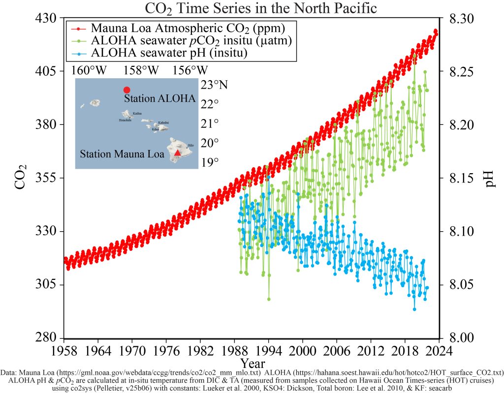
About 26% of anthropogenic carbon dioxide ends up in the oceans, where it produces and HCO3– (bicarbonate ions) and H+ (hydrogen ions:- in reality combined with water as H3O+ hydronium ions). This increases the acidity of the oceans. Ocean pH, typically around 8.1, has fallen by about 0.05 in the 30 years since precise systematic measurements became available. Although this sounds small, the pH scale is a logarithmic scale, so this represents a 12% increase in the abundance of hydronium ions. For organisms that secrete skeletons — shells etc. — of calcium carbonate this is bad news, as extra work has to be done to extract the necessary ions from sea water. For corals, this adds to the challenge of living in very warm waters, that leads to phenomena like coral ‘bleaching’ – the loss of coloured living material from the surface of the white coral skeleton.
The future
Predicting the future is difficult, but it is clear that large parts of the Biosphere, including humanity, face major challenges as a result of anthropogenic climate change.
Despite many uncertainties about the climate system, the basic science is simple, and has been uncerstood since the 1800s. The impacts of humans on the Earth system are already apparent and will accelerate without collective intervention. Avenues for intervention include:
- Reducing human dependency on energy
- Reducing the proportion of human energy use from fossil fuels, relative to other sources
- Reducing the proportion of human energy use from the most carbon-intensive fossil fuels (e.g. coal)
- Sequestering (trapping) of greenhouse gas in the Biosphere or the Geosphere.
Scientific investigations of climate have been quite successful at predicting change to this point. We have the scientific basis to understand and face these challenges, but reducing total emissions has been an elusive goal in the face of short-term economic interests. In some cases, humans have been able to work in collaboration (rather than competition) to solve collective problems. The reduction in emissions of chloro-fluoro-carbons to protect the ozone layer has been a successful example of international collaboration. Avoiding a climate catastrophe depends on finding a similar solution for the bulk of greenhouse gas emissions.
- The abbreviation CE stands for "common era" and is used in preference to the synonymous but Christianity-centric "AD". ↵
- Shaw, J., Amos, C.L., Greenberg, D.A., O’Reilly, C.T., Parrott, D.R., and Patton, E., 2010, Catastrophic tidal expansion in the Bay of Fundy, Canada: Canadian Journal of Earth Sciences, 47, 1079–1091, doi:10.1139/E10-046 ↵
- A forcing should not be confused with a force. A forcing is a factor that changes the rate of movement of energy or some substance in a cycle. A force is a quantity in mechanics that describes rate of change of momentum, or mass times acceleration. ↵
- The diagrams that follow are based on those of Kump and others 2010, The Earth System, 3rd edition. Pearson ↵
- The wording on change is important. It's not sufficient just to compare incoming radiation with outgoing heat, because the outgoing heat includes geothermal energy and tidal energy that did not come from the Sun. Radiative forcing involves only that portion of the solar energy that is added to the atmosphere rather than being radiated back into space. ↵
- Data from 6th IPCC report, 2021 ↵
Long-term trends in Earth’s atmosphere which may affect weather, but take effect for much longer. Climate is weather averaged over periods longer than a single year
Generated by humans
Information that is not a direct measurement of a physical quantity such as temperature, but which allows the value of that physical quantity to be estimated.
A short period of cooling from 1400 to 1850 CE. The little ice age was not a true glacial interval, but rather a temporary decline in temperatures across the world.
Cylindrical structures developed in the woody stems of trees, typically one per year
Fossils requiring magnification for study; fossils too small for the unaided eye to see features.
Fossils large enough to be viewed by the unaided eye.
Microscopic grains containing the male reproductive cells of plants, dispersed through air or by pollinating insects
A diverse group of marine single-celled organisms whose preserved exoskeletons (or tests) may be preserved as fossils in marine sediments.
Changes in the characteristics of organisms, and the Biosphere as a whole, over periods of many generations.
Isotopes of an element are atoms that have the same atomic number but different atomic mass, because of different numbers of neutrons in the nucleus
Atomic weight (relative atomic mass): The mass of an atom expressed on relative a scale in which the most common isotope of Carbon is given a value 12.
The tendency of unstable isotopes to decay and release radioactive particles and gamma rays.
An isotope that is able to persist over long periods of time without decay
A hydrogen isotope with an atomic mass number of 2, in which each atom contains one proton and one neutron, represented 2H or D
Cylindrical samples of glaciers acquired by drilling.
A gas in which each molecule combines one atom of carbon with two of oxygen; formula: CO2
A gaseous compound of carbon and hydrogen CH4. Methane is the principal component of natural gas. In the Earth's atmosphere it acts as a greenhouse gas.
An interval during an ice age where warmer temperatures cause worldwide glacial retreat.
A warm state of Earth’s climate, without continental ice sheets.
The Earth’s climatic state during times of cyclic expansion and retreat of ice sheets.
Lithified till: Unsorted sediments deposited directly from glacier ice, subsequently solidified
Unsorted sediments deposited directly from glacier ice
Pertaining to ice or glaciers. During cold episodes of Earth history, glacial periods are periods of more ice cover.
A climate state in which a majority of the Earth's surface is covered with snow or ice. Snowball Earth conditions are believed to have occurred during several intervals in the Proterozoic Eon.
The proportion of light that is reflected from the surface of a substance
A supercontinent assembled during the Proterozoic Eon, that was incorporated in the larger supercontinent Pangea during the Paleozoic Era. Parts of Gondwana form modern South America, Africa, Antarctica, Australia, and India.
An era in the Phanerozoic Eon of Earth history, from about 200 Ma to about 65 Ma
The current era in geologic time from ~65 Ma to the present day.
The most recent and current period of the Cenozoic Era, beginning about 2.6 million years ago. The Quaternary included significant glacial and interglacial intervals.
Repetitive variations in the Earth’s tilt, axis orientation and elliptical orbit shape, that cause climate forcing.
The angle at which the Earth’s axis of rotation is tilted towards the ecliptic.
The rotation of the Earth’s tilted axis of rotation, which causes a change in the position and timing timing of the solstices and equinoxes relative to the axes of the Earth's elliptical orbit
A time about 20 thousand years ago when glaciers reached a maximum extent.
A dimmer patch on the photosphere of the Sun associated with magnetic storms
Matter (plasma specifically) released from the surface of the Sun that carries small amounts of energy throughout the solar system.
The year 1816 CE; a short-term cooling in climate occurred during the growing seasons of the Northern Hemisphere, possibly due to the long-term effects of a volcanic eruption of Mount Tambora, Indonesia
The plate tectonic process whereby one plate descends beneath another as plates converge
Warming of the central and east Pacific Ocean surface resulting in the supression of normal December upwelling off the coast of South America
A low pressure band in the Earth’s atmosphere lying approximately along the equator
The net transport of water at 90 degrees an the original wind direction as a result of the Coriolis effect.
A phase of El Niño southern oscillation (ENSO) in which west-Pacific rise of air is intensified and the equatorial east Pacific is unusually cold
El Niño southern oscillation (ENSO) is an oscillating behaviour of the atmosphere–ocean system defined by changes in the temperature of east-Pacific surface waters over periods of several years
A system without a net flux of materials in or out; a steady state describes a system that remains unchanging over time.
The combined processes by which water is transferred from liquid at Earth’s surface to vapour in the atmosphere, comprising both physical evaporation and transpiration by plants
An effect that changes the balance of fluxes in a system and therefore cause the system to depart from a steady state
The transfer of energy through the various spheres and systems of the Earth
The process whereby a change in one part of a cycle causes changes throughout the cycle, which then affect the part originally changed
A cycle in which the products of a process act as inputs inhibiting the same process, reducing the effects of the process.
A cycle in which the products of a process act as inputs increasing the activity of the same process
A compounds in the Earth’s atmosphere which absorbs infra-red radiation, preventing or delaying its escape into space.
A collection of ecosystems having similar characteristics of climate, terrain, and energy flow
Openings on plant leaves that allow plants to exchange gases with their surroundings
The process by which igneous, sedimentary, and metamorphic rocks arise through cycling of material through the Earth's outer layers
A process whereby the chemical weathering of silicate minerals to form carbonate minerals controls the amount of silica, carbonate, and carbon dioxide in the Hydrosphere and Atmosphere.
The eon before the Phanerozoic, from 2500 to about 539 Ma, during which atmospheric oxygenation, the evolution of multicellular organisms, and Snowball Earth conditions occurred.
The third planet from the Sun known for its similar size to Earth; the brightest planet in Earth's night sky
A portion of the universe that can be regarded as separate from its surroundings for some scientific purpose.
Regions of the Earth where large amounts of magma (usually mafic) have been generated in a geologically short time.
A rigid, moving part of the Lithosphere
The movement of water currents throughout the oceans as a consequence of differemces om temperature and salinity
Elevated regions on the ocean floor centred on divergent plate boundaries.
An area of shallow sea (<200 m) at the edge of a continent, underlain by continental crust.
A mountain-building process that occurs as crust shortens during the convergence of the lithosphere.
A region of dry conditions on the downwind side of a mountain belt, due to precipitation of moisture as air moves over the mountains.
The production of reduced carbon compounds from water and carbon dioxide using light as an energy source, carried out by cyanobacteria, many algae, and plants.
The absorbtion of outgoing infra-red radiation by atmospheric gases, leading to heading of the Earth’s atmosphere.
The solar energy flux, typically measured as a rate of energy flow per square metre at the top of the Earth's atmosphere
The 11 year-long rise and fall in sunspot activity across the surface of the Sun, associated with a minor change in irradiance
An interval during the late 17th to early 18th century CE when sunspots were at a minimum
A positive feedback wherein the melting of ice reduces the albedo of Earth’s surface, allowing further warming and additional ice melting.
The length of the long axis in relation to the length of the short axis of an ellipse; a measure of the difference between the ellipse and a perfect circle.
The first era of the Phanerozoic Eon, in which multicellular organisms prominently radiated in the Cambrian Explosion, and multicellular life emerged onto land
Material near the Geosphere surface that remains frozen for two or more years.
A gas composed of nitrogen and oxygen, produced as part of the nitrogen cycle, which acts as a greenhouse gas in the atmosphere; N₂O
A compound consisting of three oxygen atoms O3 which exists in small amounts in the atmosphere due to both natural and anthropogenic activity.
The effect of carbon dioxide on the absorption and reflection of solar irradiance as it reaches Earth’s atmosphere.
Computer models for the atmosphere which which work as hypotheses for predictions about future weather and climate.
The application of historical data to a climate model in order to test the predictive ability of the model against present observations
A positive feedback phenomenon whereby more of the effect of climate change is felt in Arctic or Antarctic latitudes than is felt at the equator.
Loss of ice from a glacier
Gain of ice in a glacier
The movement of the terminus of a glacier in the opposite direction to ice flow, so that less land is progressively covered by ice; Typically occurs when ablation exceeds accumulation.
The rise of air as wind blows over hills or mountains
Local rise in sea level along a coast beneath a major storm due to the combined effect of onshore wind and reduced air pressure
A cyclonic storm that develops north or south of the intertropical convergence zone. A storm must achieve a windspeed >120 km/hr to be considered a tropical cyclone.
A negatively charged ion with the formula HCO3-, or a compound containing such ions
A positively charged ion H3O⁺ formed by the addition of a positive hydrogen ion to a molecule of water.
The standard scale of a substance’s acidity or alkalinity; minus the logarithmic concentration of hydrogen ions; acids have low pH; alkalis (bases) have high pH.
Compound with the formula CaCO3, the main component of limestone and the shells of marine
animals
The Earth system that comprises all living things and their non-living remains
