
Theoretical Foundation
Species-level conservation is fundamentally concerned with the processes governing population dynamics and how they are affected by external factors. Knowledge of these processes is gained through observational studies and demographic modelling. Models are tools that:
- Provide an organizing framework for the observational data we collect
- Allow us to explore the dynamics of the system, helping us to understand it more fully and to extract important principles
- Help us identify which parameters are most influential and where key uncertainties lie
- Allow us to make predictions about how the system will respond to alternative management scenarios
Some models are strategic in nature, sacrificing detail for generality. By incorporating relatively simple mechanisms that do not consider the details of any one system, they aim to capture the essential behaviour of many systems (Yodzis 1989). In this section, we will explore the theoretical insights fundamental to species-level conservation provided by strategic modelling. We will begin with the simplest of systems and then progressively add detail. In a later section, we will turn to tactical models, which capture the details of specific systems and are used as tools to support applied conservation.
Box 6.2. Species and Populations
For biologists, a species is a group of organisms capable of interbreeding under natural conditions. However, under SARA, “wildlife species means a species, subspecies, variety or geographically or genetically distinct population of animal, plant or other organism, other than a bacterium or virus, that is wild by nature” (GOC 2002, Sec. 2.1).
Much of the research and management that occurs under the heading of species conservation actually targets populations. A population is a group of organisms of the same species that live in a particular geographical area and which normally breed with one another. In practice, the level of interbreeding is usually unknown, and the term “population” is simply applied to local assemblages of individuals of the same species.
Insights from Simple Population Models
Every species has an intrinsic reproductive capacity, determined by the age at first reproduction, number of offspring per reproductive cycle, number of cycles per year, and so forth. Similarly, each species has an intrinsic rate of senescence that determines the maximum lifespan of individuals. Together, these two variables define the maximum population growth rate of a species.
In real-world settings, the maximum rate of population growth is rarely observed because reproduction and mortality are affected by a wide range of limiting factors. Common examples include competition for resources, consumption/predation, disease, and environmental disturbances. Some factors have a proportionately greater effect as population density increases. For example, competition for resources may be minor concern when a population is small, but a major limiting factor if its density becomes high. These are called density-dependent factors, and they serve as negative feedback mechanisms. Other factors, such as fire, have roughly the same proportional effect on populations, regardless of population density. These are called density-independent factors (Hayes et al. 1996).
A simplified illustration of density-dependent relationships is shown in Fig. 6.1. The growth rate of the entire population (total births minus total deaths) relative to density is provided in Fig. 6.2. The exact shape of these curves will vary from species to species and among regions because they depend on intrinsic species traits and the nature of the limiting factors in a given area. However, the general features of density-dependent population growth are widely applicable.
 |
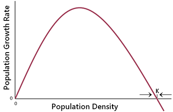 |
| Fig. 6.1. Per capita birth rate and death rate as a function of population density, illustrating simple density-dependent relationships. | Fig. 6.2. Population growth rate as a function of population density, given the functional relationships shown in Fig. 6.1. |
An important feature of these curves is that there exists a point, labelled K in Fig. 6.1, where the population is in equilibrium because the rate of births equals the rate of deaths. The point K is usually referred to as the carrying capacity (Yodzis 1989). Because of density-dependent feedback processes, the population will intrinsically revert back to K if it is perturbed (see Fig. 6.2). As such, K is an important point of reference for management.
The Natural Range of Variability
In our simple example, population size becomes static once the density equals the carrying capacity. But real-world populations tend to fluctuate in size because many of the factors that influence reproduction and mortality are intrinsically stochastic (i.e., exhibit randomness). Sporadic disturbances and environmental processes with inherent variability, such as weather, have the greatest effect (Lande 1993).
The time it takes a population to return to its equilibrium state after a perturbation is a measure of its resilience (Gunderson 2000). This rate is determined by the population growth functions we discussed earlier (Fig. 6.2). Under natural conditions, a population’s resilience is generally sufficient to accommodate the disturbances it encounters, and so it fluctuates about its equilibrium value (Fig. 6.3). Species unable to accommodate such perturbations are eliminated through natural selection.
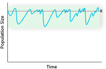
Given the stochasticity inherent in population dynamics, it is difficult to determine carrying capacity through direct observation. The natural range of variability (NRV) is often used instead as the reference state for management (Fig. 6.3). In areas where natural conditions prevail, the NRV of a given population can be determined through long-term monitoring. For populations in developed areas, NRV can be derived from historical data, extrapolated from nearby natural areas, or estimated using population models. Because of data limitations, only a rough estimate may be possible in such cases.
Population Decline
Having explored the dynamic processes characteristic of natural systems, which feature fluctuations about an equilibrium point, we now turn to the processes involved in systematic population decline (Caughley 1994). A widespread cause of population decline is habitat loss. Individuals that are displaced through habitat loss cannot simply crowd into the remaining habitat because it cannot support a density greater than the carrying capacity, at least not for long. Therefore, losses in habitat area translate into direct losses in overall population size.
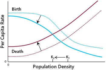
Population decline can also occur because of changes in per capita birth and death rates (Fig. 6.4). The list of proximate causes includes overharvesting, reduction in habitat quality, competition from alien species, pollution, and various other factors (detailed in Chapter 5). To understand the population dynamic implications, it does not matter too much whether birth rates decline or deaths rates increase (or both). The main consequences are a reduction in the intrinsic population growth rate and a lower carrying capacity (K2 in Fig. 6.4).
A reduction in the population growth rate can result in a range of outcomes (Hayes et al. 1996). In the extreme case, where mortality exceeds reproduction at all densities (implying a negative growth rate), the population will invariably go extinct. Large initial population size may slow the process, but will not prevent it, as illustrated by the extirpation of Canada’s plains bison from overhunting.
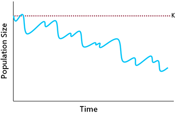
If the intrinsic growth rate remains at least somewhat positive, the long-term outcome depends on the balance between the rate of population growth and the rate of environmental disturbances. Given sufficient growth potential, a population can recover from disturbances and remain within NRV. However, beyond a certain point, the rate of recovery may become too slow to keep pace with disturbances, resulting in a declining trend (Fig. 6.5).
Changes in the birth rate and death rate can also lead to a reduction in carrying capacity (Fig. 6. 4). If this happens, the population will equilibrate at a lower density, assuming that the growth rate is sufficient to maintain stability (Fig. 6.6). The danger here is that, if the new equilibrium density is very low, extinction may result from the demographic challenges of small populations (discussed below).
 |
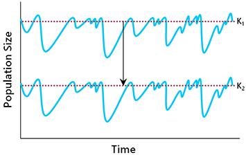 |
| Fig. 6.5. If a population’s intrinsic growth rate declines, it may be unable to recover quickly enough from periodic environmental disturbances to prevent a declining trend. | Fig. 6.6. When K is reduced, the population will equilibrate at a lower density, potentially exposing it to the demographic challenges of small populations. |
In some cases, declining trends can be reversed through remediation of the inciting causes, allowing populations to re-establish their original NRV. For example, by banning DDT, hunting, and egg collecting, peregrine falcon growth rates have been substantially restored, and populations are now recovering (albeit, with initial help from captive breeding programs; COSEWIC 2007).
More commonly, mitigation efforts are constrained by socio-economic trade-offs that preclude full recovery (Traill et al. 2010). For example, plains bison have sufficient growth potential to return to their original NRV. But such recovery would require the naturalization of vast landscapes now used for agriculture, which is politically infeasible. We will explore these sorts of trade-offs later in the chapter.
Ecological Thresholds

In some cases, a species may exhibit a linear response to a given environmental driver (Fig. 6.7). For example, population size may decrease in direct proportion to the amount of habitat loss. More commonly, a species may show little response to low levels of the driver and then, at a certain point, exhibit a disproportionately large response. This transition point is referred to as an ecological threshold, and it results from nonlinear system dynamics (Kelly et al. 2015).
An ecological threshold is typically observed when compensatory processes initially buffer the effect of an environmental driver. The driver’s ecological effects become apparent once this buffering capacity is exceeded. For example, given a population at carrying capacity, harvesting at low levels may simply offset other forms of density-dependent control, whereas harvesting at higher levels may exceed the capacity for compensation and result in population decline (Boyce et al. 1999).
Though ecological thresholds are undoubtedly common in natural systems, they are difficult to quantify. Data must be collected across a broad range of disturbance levels, which is not always possible. Interactions with other drivers and ecological inertia can also complicate matters (van der Hoek et al. 2015).
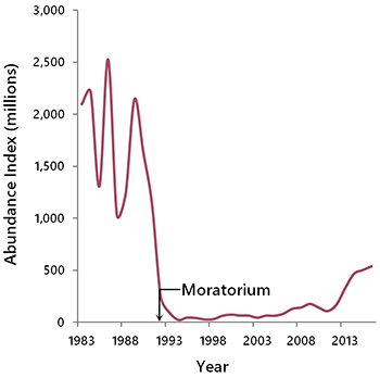
When an ecological threshold can be reliably delineated, it facilitates the selection of management targets. In cases where ecological responses have not been well described, a linear relationship is usually assumed. In some cases, an ecological system may undergo qualitative changes once a species declines below a certain point, making recovery much more difficult (Gardmark et al. 2015). This is another form of ecological threshold. Northern cod provide an example. Intensive harvesting of cod released herring from predator control, leading to an altered ecosystem (Fauchald 2010). In this new state, an abnormally large population of herring suppressed cod recruitment through predation on cod eggs and larvae. Consequently, the path to cod recovery has been prolonged, despite the moratorium on fishing implemented in 1992 (Fig. 6.8).
Box 6.3. Traits that Predispose Species to Extinction
Several species traits are associated with an increased risk of extinction, either because they increase exposure to anthropogenic threats, or because they hinder the ability of a species to cope with these threats (Flather et al. 2011). It is worth noting that large mammals exhibit many of these traits, partially explaining their prominence as focal species (Carroll et al. 2003). Traits predisposing to extinction include:
- Reproductive strategies designed for stable environments, including late maturation, low reproductive potential, and low natural density
- Large body size and large home range size
- Habitat or diet specialization, particularly if associated with a restricted range
- Commercial value (e.g., for hunting or fishing)
- High sensitivity to common anthropogenic effects (e.g., vulnerability to pesticides)
- Long-range migration
- Colonial nesting
Extinction Dynamics
Once populations become small, the extinction risks from stochastic processes are magnified, and genetic and demographic factors also become important (Caughley 1994). The population threshold at which these processes become a serious concern varies by species and individual circumstances. However, we can use generic estimates derived from theoretical analyses to convey the relative importance of the mechanisms involved.
Environmental stochasticity is the most significant factor involved in extinction dynamics because it includes catastrophic events, like large fires, that can cause the direct mortality of large numbers of individuals (Lande 1993). Small populations face the highest risk because even relatively small disruptions can result in extinction (compare the two populations in Fig. 6.6). As a ballpark estimate, achieving long-term persistence in the face of environmental stochasticity may require a population of several thousand individuals (Soule 1987; Traill et al. 2010).
Genetic effects contribute to extinction risk in two main ways. Once populations become small (less than ~1,000 individuals) any further loss of individuals may result in the loss of genetic variability (Shaffer 1981; Lande and Barrowclough 1987). This reduces the capacity of individuals and populations to adapt to changing conditions. At even lower population sizes (i.e., less than approximately 50 reproductive individuals) the fitness of individuals may be further reduced through inbreeding depression (Saccheri et al. 1998). Inbreeding depression involves the increased expression of recessive deleterious mutations from mating among genetically related individuals in small populations (Charlesworth and Willis 2009).
Populations less than approximately 100 individuals also face extinction risk from demographic stochasticity. This arises from fluctuating sex ratios, random variation in the number of offspring produced, and chance mortality events (Lee et al. 2011). In large populations, such randomness is averaged out across individuals and has no discernible effect. But when only a small number of individuals remain, chance occurrences, like a string of all male offspring, can significantly affect demographics.
Finally, in some species, extinction dynamics are influenced by Allee effects, which are cooperative group processes that facilitate population growth (Boukal and Berec 2002). Examples include communal defence against predators, communal raising of offspring, and efficient mate finding. When populations that depend on Allee effects become too small for group processes to operate, population growth rates can quickly decline, reducing viability.
Box 6.4. Extinction Vortices: the Case of the Heath Hen
The various demographic and genetic processes that affect small populations often operate synergistically, causing an extinction vortex. The extinction of the heath hen, as recounted by Shaffer (1981), provides an illustrative example. The heath hen was a type of prairie chicken originally found in the northeastern US. Once common, its abundance steadily declined with European settlement as a result of habitat loss and increased mortality (i.e., systematic decline). By 1876, the species remained only on Martha’s Vineyard, and by 1900 there were fewer than 100 survivors. In 1907, a portion of the island was set aside as a refuge for the birds, and a program of predator control was instituted. The population responded to these measures and by 1916 had reached a size of more than 800 birds. But in that year, a fire (natural catastrophe) destroyed most of the remaining nests and habitat, and during the following winter, the birds suffered unusually heavy predation from a high concentration of goshawks (environmental stochasticity). The combined effects of these events reduced the population to 100–150 individuals. In 1920, after the population had increased to about 200, disease (environmental stochasticity) took its toll, and the population was again reduced below 100. In the final stages of the population’s decline, the birds appeared to become increasingly sterile, and the proportion of males increased (demographic stochasticity and inbreeding). By 1932, the species was extinct.
Spatially Structured Populations
To this point, we have implicitly assumed that populations exist in simple homogenous landscapes. We will now consider the dynamics of populations in more realistic environments, where habitat quality varies across space.
In a heterogeneous landscape, the various limiting factors that influence reproduction and mortality will vary from location to location. Thus, population densities will also be spatially variable. In the absence of immigration, we can expect populations to persist only in areas where the carrying capacity is greater than zero.
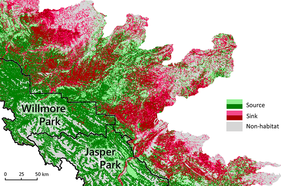
Population dynamics are more complex when immigration and emigration are included in the system. We must now differentiate between source habitats—areas where intrinsic growth is sufficient to maintain viability—and sink habitats—areas where populations are only able to persist through immigration from source populations (Fig. 6.9; Pulliam and Danielson 1991). Though sink habitats cannot support populations independently, they still contribute to overall species viability. They expand the range of the species and increase overall abundance, both of which help to buffer against environmental stochasticity (Carroll et al. 2003).
For some species, habitat is perceived as discrete patches. For example, the scattered sloughs in a prairie landscape constitute discrete habitat patches for frogs and other wetland species. If the patches are sufficiently isolated from each other, a population may be divided into subpopulations that exhibit semi-independent dynamics. In this case, the assemblage of subpopulations is referred to as a metapopulation (Hanski 1998).
If the patches of habitat are relatively small, the individual subpopulations may be vulnerable to decline or extinction from the stochastic and genetic processes we discussed earlier (Hanski 1998). But there also exists the possibility for rescue through emigration from neighbouring subpopulations. The overall metapopulation is said to be in an equilibrium state when the processes of loss and rescue are in balance. The main parameters influencing these dynamics include:
- Patch size. Large patches are more stable and produce more migrants.
- Degree of environmental synchrony among patches. The potential for rescue improves when patches do not experience the same pattern of fluctuations.
- Dispersal ability. Movement is affected by species-specific dispersal traits and by the permeability of the non-habitat matrix.
- Distance between patches. Longer distances reduce the number of immigrants, but also reduce the level of environmental correlation, so the effects on viability are complex.
In natural landscapes, species that exhibit metapopulation dynamics normally have sufficient dispersal ability to keep subpopulation decline and rescue in balance and to maintain gene flow. Again, natural selection has long ago weeded out species unable to do so. However, anthropogenic disturbance can easily disrupt this equilibrium, either by reducing the viability of individual subpopulations or by changing the permeability of the matrix (Mennechez et al. 2003).
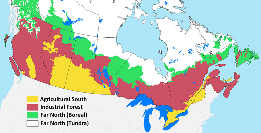
Human development also can produce metapopulations artificially, by fragmenting the habitat of previously continuous populations (Fig. 6.10). This has occurred extensively in the Agricultural South (Fig. 5.5). The viability of such nouveau metapopulations is not guaranteed because connectivity among remnant patches may be low under such artificial conditions, at least for some species (Tucker et al. 2018).

Species Range
The range of a species is the overall geographical area in which its populations are found. In the simplest case, where limiting factors exist as uniform gradients, we would expect a species to be most abundant in the centre of its range and progressively decline toward the periphery. However, limiting factors in real landscapes often exhibit non-uniform patterns; therefore, species distributions are typically quite complex (Sexton et al. 2009; Boakes et al. 2018). Gaps in distribution may exist within the range, and the centre need not have the highest abundance (Gaston 2009).
Range boundaries are also influenced by the interplay between dispersal and environmental stochasticity (Hargreaves et al. 2014). If environmental variability is low, species may routinely occupy sink habitat in peripheral regions through ongoing emigration from source habitat. Conversely, in the face of high environmental stochasticity and low dispersal ability, areas where the carrying capacity is only marginally positive may be unoccupied. Because of these processes, fragmentation of population structure is common along range margins.
Limiting factors may systematically change over time, redefining the region in which populations can persist. Human disturbances have been the main driver of such systematic changes, leading to widespread range contractions in many species (Channell and Lomolino 2000). More recently, ranges have begun to shift as a result of climate change. In this case, all species are affected (see Chapter 9).
When environmental conditions undergo systematic change (regardless of the cause), population responses may lag behind. Disequilibrium is most likely to occur in species with long generation times (e.g., trees) and when the pace of environmental change is rapid. In the case of deteriorating conditions, demographic lags may result in populations that continue to exist while on an extinction trajectory. Such populations represent an extinction debt (Kuussaari et al. 2009).
