
Tactical Modelling
The general principles that have emerged through strategic modelling form the foundation of species-level conservation. But broad concepts and principles can only go so far. Applied conservation also requires attention to the unique characteristics of individual populations in real landscapes, especially for the assessment of risk and the efficient allocation of conservation efforts. This is the purview of field research and associated tactical models. Not all conservation practitioners will be directly involved in conducting field studies and modelling, but most will be users of the information provided and need to be able to assess it critically and apply it effectively.
Most tactical models are statistical models that mathematically summarize important patterns and relationships in the data generated by individual observational studies. Tactical models can also be constructed by combining the findings from multiple observational studies into a composite process-based model. Both approaches are used in applied settings to generate predictions that support management decisions. These models also can identify the factors that are most influential in a system and pinpoint where key uncertainties lie. This information provides guidance for future field research and helps managers understand the reliability of the predictions being made.
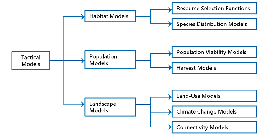
There are three main categories of tactical models (Fig. 6.11):
1. Habitat models, for the study of habitat selection and species distribution
2. Population models, for the investigation of population dynamics and viability
3. Landscape models, for the study of connectivity patterns and the exploration of population responses to landscape changes from anthropogenic disturbance and climate change
In practice, hybridization among these model categories is common, and arguably essential in many applications. But for the sake of clarity, we will treat the various modelling categories as discrete entities, emphasizing the intended purpose of each approach and its main assumptions and limitations. In the case studies presented in Chapter 11, we will see how tactical models are used in real-world applications.
Habitat Models
Habitat models are used to gain insight into the basic ecology of a species and to make predictions that inform management. At the local scale, the main interest is identifying the habitat types that are most important to a species so they can be maintained through management prescriptions and guidelines.
At broader scales, the main interest is in identifying geographic regions that feature high-quality habitat. This information is used to select optimal sites for species reintroductions and for the establishment of protected areas (e.g., Nielsen 2006). It also can inform the designation of critical habitat under SARA (see below). Habitat studies are also integral to determining range extent and range trends, which are often incorporated into status assessments and management targets (Loehle and Sleep 2015).
Most habitat modelling involves the statistical extrapolation of data collected in observational field studies (Lele et al. 2013). Statistical approaches are used because it is generally not feasible to study all individuals in a population. We sample a subset of the population and then use models to infer habitat relationships for the entire population.
The data for statistical habitat models are collected in a variety of ways. A common approach is to survey usage along transects or at specified locations. Usage is determined by visual sighting (e.g., aerial surveys of large mammals), auditory detection (e.g., breeding bird surveys) and evidence of recent use (e.g., snow tracking). In recent years, camera traps, acoustic recorders, and DNA markers have greatly augmented the collection of survey data (Steenweg et al. 2017).
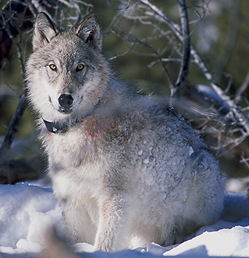
Another common approach for collecting usage data is to track the movement of individuals using attached location transmitters (Fig. 6.12). In the past, these transmitters emitted radio signals that required manual relocations to be made using portable antennas. More recently, tracking devices have been developed that automatically take GPS locations at timed intervals, providing much greater detail on movement paths (Hebblewhite and Haydon 2010).
To determine habitat associations, data also must be collected on relevant environmental variables. Our ability to do this effectively has undergone tremendous improvement over the last two decades, with the advent of geographic information systems (GIS) and multi-layered spatial datasets. By documenting the distribution of habitat types across the entire study area, it is possible to determine not only which habitat types are being used, but which are being actively selected. We say that a habitat type is being selected if its proportional use exceeds its availability in the study area (Aarts et al. 2012; Boyce et al. 2016).
Analytical approaches have evolved alongside advances in data collection and data processing. The relevant approaches fall into two main categories. Resource selection functions (Lele et al. 2013) explain and predict habitat selection by individuals at the local scale, and species distribution models (Elith and Leathwick 2009) explain and predict patterns of species occurrences at broad scales. The statistical methods used by these two approaches are broadly shared, so it is mainly scale and purpose that differentiate them (Aarts et al. 2012). Newer approaches, such as step selection functions, have been developed to handle the large amounts of data being generated in GPS-based tracking studies (Thurfjell et al. 2014).
An older form of habitat modeling, widely used in the twentieth century, is habitat suitability index modelling, a quasi-mechanistic approach (Schamberger et al. 1982). The development of these models begins with a review of the literature to identify the habitat variables most strongly related to population dynamics of the species of interest. Using expert opinion, these variables are then qualitatively combined into an equation that provides an index of habitat quality. Today, quantitative statistical approaches are preferred; however, habitat suitability index modelling still has a role in cases where the detailed datasets needed for quantitative analysis have not or cannot be collected (e.g., Stevens et al. 2008).
All forms of habitat modelling are subject to various limitations that users of the results need to consider. There are three main areas of concern: reliability of estimation, differences between habitat selection and habitat importance, and inappropriate extrapolation.
Problems with reliability arise from the challenges inherent in sampling biological systems. Depending on the species, habitat associations may vary by age, sex, season, and year (Alldredge and Griswold 2006). Relationships also can be affected by habitat availability and its distribution, since animals can only select from what is on offer (and this might not include what is most desired). In addition, observed associations can be influenced by detection biases and by errors in the classification of environmental variables (Wilson et al. 2005; Burton et al. 2015). The latter is a common problem when satellite imagery is used to specify vegetation types (Rocchini et al. 2013). If these potential sources of variability and bias are not addressed through appropriate sampling design (MacKenzie and Royle 2005), the model will not provide a reliable representation of the system.
A second limitation of habitat models is that selection is not necessarily indicative of importance to demography (Alldredge and Griswold 2006). Much depends on how the environmental variables are specified. If habitat variables are poorly defined, important relationships may be overlooked. Furthermore, some critical habitats, such those required for nesting, may only be used for limited periods, which can lead to an underestimation of their importance (Alldredge and Griswold 2006).
At broader scales, the interpretation of selection studies may be complicated by demographic processes (Boyce et al. 2016). High-quality habitats might be unused for reasons unrelated to habitat conditions, such as overhunting. Conversely, immigration into sink habitats may result in an overestimation of their value. Consequently, the interpretation of habitat value from selection studies should be done in conjunction with knowledge about the basic ecology of a species.
Finally, as with all statistical models, there are limits to extrapolation. Predictions of habitat use applied within the study area itself are usually sufficiently reliable for decision making as long as no major changes occur in the system (Elith and Leathwick 2009). However, when extrapolating to external regions or to future periods, reliability is unknown.
A key concern is that habitat availability often varies among regions and time periods, and this can influence selection patterns. For example, Canada warblers in New Hampshire select red maple swamp, dominated by red maple, balsam fir, and red spruce, whereas those in the western Canadian boreal forest select old-growth aspen and aspen-spruce mixedwoods (EC 2016). Choices are also influenced by biotic interactions, which may not be constant over space and time (Elith and Leathwick 2009). In the future, as temperatures rise, different rates of northward migration may result in novel species interactions that influence competition and habitat use in new ways (Williams and Jackson 2007).
One solution for predicting habitat selection across larger areas is to expand the study area and another is to create separate regional models (Wiens et al. 2008). The latter is more common because it does not require any sacrifice of detail, and because smaller studies are easier to fund and coordinate. As for modelling future periods, we will discuss the relevant approaches in Chapter 9, in the context of climate adaptation.
Box 6.5. Ecological Niche
A species’ niche can be defined as the range of biotic and abiotic conditions within which its populations can persist without immigration (Araujo and Guisan 2006; Wiens et al. 2010). The conditions being referred to here are related to the limiting factors for population growth we discussed earlier, indicating a direct connection between ecological niche and demography.
There is also a connection between niche and habitat. Niche refers to the set of conditions that support existence, and habitat refers to the physical locations where those conditions can be found. This distinction is fairly nuanced, and consequently the terms are often used interchangeably (Whittaker et al. 1973).
A species’ tolerance to individual limiting factors, such as temperature, will often be broader than its observed distribution suggests. This is because a species will only occur where all of its essential parameters are within acceptable limits. Moreover, distributions are strongly influenced by competition and other biotic interactions. Therefore, it is useful to differentiate between the fundamental niche of a species, referring to its complete range of tolerances, and the realized niche, which is what we actually observe. Here again, there is a lack of consistency in the criteria used for making this distinction (Araujo and Guisan 2006).
In conservation applications, we are mainly concerned with the realized niche. Strictly speaking, the realized niche includes anthropogenic disturbances as a limiting factor. However, in practice, it is common to differentiate the ecological niche that exists under natural conditions from the niche that is realized in landscapes impacted by humans.
The term “ecological niche” is also used to describe the functional role of a species within a community, particularly in relation to its food and enemies. In this usage, a species’ niche is seen as a collection of structural, physiological, and behavioural adaptations that has evolved in the context of competition with other species. This form of niche is associated with the concept of competitive exclusion, which posits that no two species can indefinitely occupy the same ecological niche, driving evolutionary differentiation (Levin 1970).
Population Models
Tactical population models were initially developed to support the management of species that are harvested. The core concept in this application is maximum sustained yield (Sissenwine 1978), in which harvest rates are tailored to achieve a population density that delivers maximal population growth (i.e., the top of the curve shown in Fig. 6.2). Such models have been used to predict the maximum sustained yield under varying environmental conditions and alternative harvest scenarios (Taylor et al. 2008).
Tactical population models are also used in the management of species at risk (Boyce 1992). Here, the emphasis is on modelling population trends with the aim of characterizing the risk of extinction, prioritizing threats, exploring alternative management approaches, and identifying key uncertainties.
In population models, abundance is a function of the population birth rate and the population death rate, often broken down by age class and sex. These two core variables are in turn influenced by other factors, such as habitat protection measures and artificial rearing. The choice of model components is based on what is relevant to the species of interest, constrained by the availability of information. In most cases, a link to habitat is warranted, but it is not always the most important factor. Knowledge gaps often stimulate additional field research, leading to later revisions of the model and evolving model complexity.
Model construction begins with a conceptual model that maps out the main components of the system and qualitatively describes the linkages between them. This conceptual model is then typically implemented as a computer simulation, which permits rapid exploration of the system’s behaviour. To run the model, the variables are parameterized using data from relevant field studies. Many models allow parameter values to fluctuate at each time step (within natural bounds) to simulate stochastic processes. Because each run produces a different result, the behaviour of stochastic models must be summarized over hundreds or thousands of runs.
As output, population models provide the predicted size of the population over time. In many cases, the raw population trend is itself of primary interest. In other cases, the emphasis is on population viability, expressed as the mean time to extinction across all runs. Viability is sometimes also expressed as the minimum viable population size, which is the minimum number of individuals required to achieve a specified probability of persistence (Shaffer 1981). This amounts to an expression of acceptable risk and requires a time period to be specified. For example, we might seek a population that has a 99% chance of surviving for the next 100 years.

In practice, population modelling is often exploratory. Parameters under management control may be run at different levels, corresponding to alternative management strategies. For example, the relationship between population trends and habitat supply might be explored by varying the amount of habitat available to the species (Fig. 6.13). Because parameter values are rarely known with precision, it is common to run the model across a range of likely values. This is known as sensitivity testing. Such testing is useful for quantifying uncertainty and identifying the parameters that are most influential. Parameters that are both influential and poorly characterized are a priority for future research.
As with habitat models, population models are subject to limitations that end-users should be aware of (Flather et al. 2011). To begin, the relationships in population models are based on correlative field studies and are subject to all the limitations of these kinds of studies.
More generally, even the most complex population models suffer from missing relationships and other knowledge gaps. Ecological data are difficult and costly to obtain, so only a subset of the factors and relationships that affect a population can be incorporated. Modellers must work with what they have and hope that the missing relationships have limited effect or are accounted for indirectly. However, it is impossible to know this with any certainty.
Given these limitations, we should not expect population models to be omniscient predictors of the future (Boyce 1992). The quantitative estimates of population size they provide are often just coarse approximations, especially in species at risk, which are generally subject to major knowledge gaps (Fieberg and Ellner 2000; Morrison et al. 2016). The main utility of these models is in providing insight into the relative importance of the threats facing a species, helping managers allocate limited conservation resources efficiently (Boyce 1992). In addition, meaningful comparisons can often be made among alternative management approaches, aiding in the identification of the most effective approach. In summary, population models allow us to consolidate what we know about a system and thereby inform management decisions, but we must remain attuned to their limitations.
Landscape Models
Landscape models are used to explore landscape connectivity and landscape dynamics. These models incorporate elements of both habitat and population models and can be thought of as an extension of these other approaches.
Landscape connectivity models are used to predict how individuals move within a given landscape. Management applications are typically focused on identifying critical movement corridors so they can be protected (see Chapter 7).
Connectivity modelling usually begins with the production of a so-called “resistance” layer, which characterizes the permeability of a given landscape to animal movement (Rudnick et al. 2012). The resistance layer is generated within a GIS by assigning different levels of permeability to landscape patches or pixels based on their composition and structure. Permeability rules may be derived from models of habitat suitability, gene flow, or individual-based movement (Rudnick et al. 2012). Alternatively, if the data required for detailed modelling are not available, permeability may be based on the level of habitat disturbance (Koen et al. 2014a).
With a resistance layer in hand, various techniques are available to identify optimal movement pathways, as well as movement pinch points that are priorities for management intervention (Rudnick et al. 2012). Least-cost path modelling has been commonly used for this purpose in the past (Rouget et al. 2006; Poor et al. 2012). Newer methods are also being employed, such as circuit theory, in which animal movements are simulated as an electric current in a resistance network (Pelletier et al. 2014; Proctor et al. 2015).
The development of a resistance layer invariably involves simplifications because detailed information on movement behaviour is difficult to obtain and because there are practical limitations on model complexity. In most cases, the resistance layer provides only a coarse approximation of how organisms move through real landscapes (Rudnick et al. 2012). For many applications, such as the identification of critical movement bottlenecks, this may suffice.
Landscape models are also used to explore the effects of landscape change on population dynamics. Some applications focus on individual species and can be considered enhanced versions of the population models we discussed earlier. The purpose of adding landscape dynamics is to increase model realism. In other applications, the emphasis is on modelling landscape changes, with the aim of supporting land-use decision making. These types of models usually incorporate sub-models to track the effects of landscape change on selected output indicators. The sub-models used to predict focal species responses are typically fairly simple.
Landscape models are also used to estimate the minimum viable area of a species, representing the geographic correlate of minimum viable population size (Brito and de Viveiros Grelle 2004). These models are subject to the limitations of population viability modelling discussed earlier.
Finally, landscape models are used to predict the effects of climate change on populations. Most applications involve bioclimatic envelope models—a form of species distribution model—to predict range shifts under alternative climate warming scenarios. Less commonly, mechanistic models are used to investigate transitional processes. We will discuss these types of models in Chapter 9.
