
22 The Tectonic System
This chapter is a near-final draft. Certain figures and glossary entries need to be added.
Learning Outcomes
By the end of this section you should be able to:
- Distinguish between the theories of continental drift and plate tectonics
- Use geophysical and geological evidence to interpret plate movement
- Identify processes characteristic of three types of plate boundary
- Spreading centres
- Subduction zones
- Transform faults
In this chapter we will look at the tectonic system: the system that has caused constant change in the Geosphere since the origin of the Earth over 4.5 billion years ago. We will begin with a look at continental drift: a theory that did not find widespread support, at least among North American and European Earth scientists, in the early part of the 20th century. We will then look at geophysical evidence that suggested that movements were possible, and which led to the theory of plate tectonics, which became a new paradigm for Earth science in the late 20th century.
In the 21st century it has become possible to observe plate movement directly, for example with the global postition system (GPS). We will conclude this section with a summary of the processes that occur at each of the three types of plate boundary, and a brief look at what is known of the forces that drive plate tectonics.
Continents and oceans
Major features of the Geosphere surface
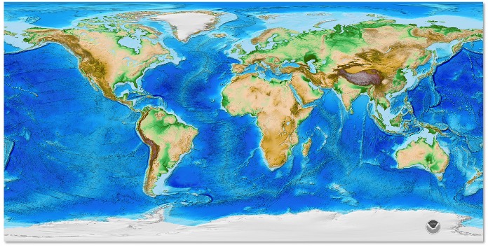
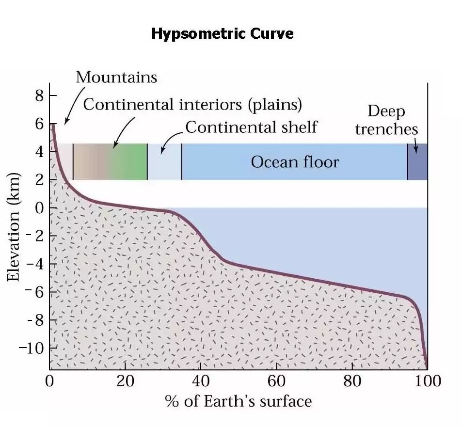
As is clear almost anywhere on the Geosphere, its surface is not level. There are major features on the surface of the Geosphere that are described as topography when on land, and as bathymetry when covered by the waters of the hydrosphere. If we look at the distribution of different elevations (a hypsometric curve), we find that there are two modes (most common values) in the distribution of elevations. Continental areas, averaging 0.8 km above sea level, and oceanic areas, averaging 3.7 km below sea level.
Samples from the continents and oceans show contrasting compositions, too. Most samples of igneous rock from the oceans are mafic in composition, whereas rocks from the surface of the continents, though extremely varied, are on average of intermediate to felsic composition.
Some other major features are apparent from the map. The continents include elongated areas that are particularly high, known as orogens. The highest point on the land surface, Mount Everest, lies in one of these, the Himalayan Orogen. There are also extensive regions on some continental margins that extend under water, but where the water is less than 200 m deep, called continental shelves. Though water-covered, these are clearly geologically continental, rather than oceanic.
The oceans include some distinctive features too. The deepest parts of the oceans are elongated troughs, up to 11 km deep, called trenches. The deepest point on the ocean floor lies in the Mariana trench in the west Pacific Ocean. Many ocean trenches are bordered on one side by curving chains of volcanoes called island arcs.
Some ocean basins, notably the Atlantic and the East Pacific, contain broad mid-ocean ridges that stand 2-3 km above the surrounding abyssal plains. Many are over a thousand kilometres wide.
Early ideas of continental drift
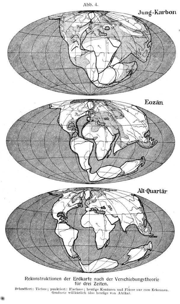
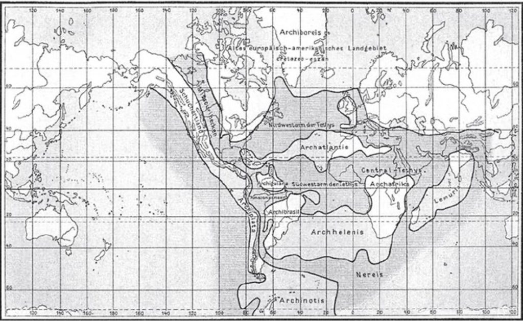
Since the development of the first global maps, many geographers have noted the match or “fit” between the coastlines of Africa, South and North America. In 1914 a German atmospheric scientist, Alfred Wegener, published his “Continental Drift” hypothesis, which suggested that the continents have moved over geological time.
Wegener’s evidence included:
- The apparent similarity of the coastlines of Africa and South America,
- Similarity of rocks on the margins of these continents, at places that would be adjacent if the continents were adjoining,
- Evidence for glaciation in places now located in the tropics,
- Remains of tropical plants in Antarctica,
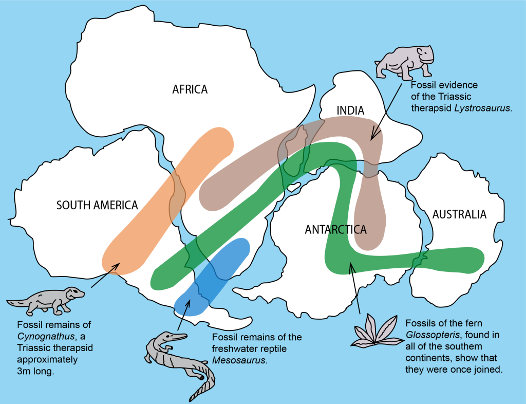
- Fossil remains of organisms that lived in restricted areas that are now widely separated geographically.
Wegener envisaged continents that move a little like icebergs through a plastic, deformable material that made up the floors of the oceans.
Although Wegener’s ideas were accepted by a few, notably in Africa and South America, most European and North American Earth scientists in the mid-20th century did not believe that continental drift had occurred. The main arguments against came from geophysics:
- Ocean floor rocks were known to be too rigid to allow continents to move;
- Seismic waves showed the mantle to be an elastic solid
To explain the similarities in fossils between the continents, it was proposed that “land bridges” extended in the past between continents that were now separated.
Ironically, the main “mobilist” arguments in favour of plate tectonics came from geophysicists in 1950s and 1960s. In the following sections we will look at each of these in turn. The first papers identifying the lithosphere, divided into plates were published between 1963 and 1968 CE, and by about 1975 most Earth scientists were convinced that continents were in motion relative to one another.
The new theory of plate tectonics differed from earlier ideas of continental drift because:
- Plate tectonics recognizes that the ocean floor is mostly rigid;
- Deformation occurs along narrow plate boundaries;
- Plates are made not just of crust but of of lithosphere – crust and upper mantle;
- A single plate may carry continental and oceanic crust.
The main lines of evidence for this new, mobile view of the Earth were derived from the study of geophysics, especially
- Gravity
- Magnetism
- Earthquakes (seismicity)
Additional early estimates of plate motions were derived from the behaviour of mid-plate volcanoes, like those in Hawai’i, located over mantle hotspots. Since around 2000 CE we have been able to measure plate motion directly using precise measurements with GPS.
Gravity, Isostasy and the Asthenosphere
Gravity
The study of gravity depends on the fact that all objects in the universe attract each other with a force proportional to their masses, and inversely proportional to the square of the distance between them (Newton’s law of gravitation). Although we like to think of Earth’s gravity as coming from one point, it actually results from the averaged attraction of all the Earth’s parts. As a result, gravity varies very slightly from place to place on the Earth; it’s stronger where dense rocks are close to the surface and weaker over less dense rocks. Measurements of the force of gravity, can be made with a gravimeter, which uses a very sensitive spring to detect very small variations in gravity. These variations, known as gravity anomalies, can tell us about the distribution of dense and less dense rocks rocks within the Geosphere.
Isostasy
The earliest systematic measurements of gravity were made by colonial surveyors in 19th-century India, who were dependent for their measurements on having a precisly vertical plumbline. Typically this was a weight hanging from a long thread. They noted that the measurements were inconstent, and realized that this was due to the extra mass in the Himalayan mountain range, to the north of India, which was deflecting the plumblines due to its gravitational attraction. They therefore attempted to correct for the mass of the Himalaya by assuming that its density was typical of crustal rocks, and found that the deflection was actually less than predicted by Newton’s law of gravitation.
Hence, they deduced that the high mountains must be underlain by less dense rocks than those that were below the plains and oceans in the area. Negative gravity anomalies, indicating less dense rocks, were found to be associated with many mountain belts. This led to the idea that mountains behave as if an upper rigid lithosphere floats on something softer below, which we now identify as the asthenosphere, rather like icebergs floating on the ocean. This idea became known as the theory of isostasy.
The concept of isostasy helps to explain some other major features of the Earth’s surface. For example, the oceans are typically floored by denser, mafic rocks whereas the continents have intermediate to felsic compositions, with lower densities. Isostasy can thus explain the contrast in elevation between continents and oceans, as the denser mafic oceanic crust “floats” at a lower level on the asthenosphere.
Isostasy can also be established in areas covered by ice caps or ice sheets. We find that the outer part of the Earth is depressed compared to surrounding areas. When an ice sheet melts we find that the outer parts of the Earth undergo isostatic rebound as the weight of ice is removed. This leads to uplift of the land relative to the sea, and phenomena like raised beaches. They don’t rebound immediately — there is a delay. The delay can actually be used to measure the viscosity of the asthenosphere.
Gravity measurements thus establish that there is a region of the Earth, the asthenosphere, which is able to flow slowly, located between about 100 and 400 km down within the mantle. Although the idea of isostasy mostly refers to vertical movements, like isostatic rebound, we now know that near-horizontal flow in the asthenosphere allows plate movement to occur. The more rigid, somewhat elastic layer above the asthenosphere, which is divided into plates, is known as the lithosphere.
Geomagnetism
The Earth’s core is the source of a strong magnetic field, known as a dipole field, that acts approximately like that of an enormous bar magnet, oriented roughly parallel to the Earth’s spin axis. This is the reason that a compass works for navigation.
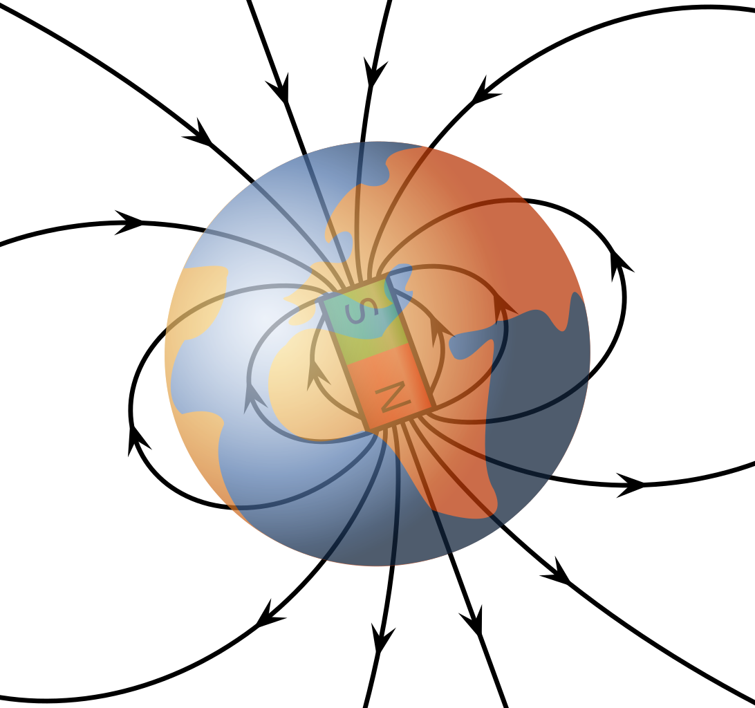
The Earth’s magnetic field also protects the biosphere from detrimental effects of the “solar wind” of particles from the Sun. Of course, there isn’t really a large bar magnet in the core! Our best efforts to model the Earth’s magnetic field suggest that it is the result of electric currents flowing in the liquid, circulating metal of the outer core.

Some of the earliest evidence in support of continental drift came from a branch of geophysics called paleomagnetism. To understand how this works we need to look a little more closely at the Earth’s magnetism.
Inclination and declination
At any place on the surface of the Earth, the magnetic field has a direction relative to north, called a declination, and it has a steepness, known as the inclination. In most places that are far from the geomagnetic poles the declination is just a few degrees east or west of north. However, the inclination can be quite steep. As a result, if we were to use just a magnetized needle as a compass for navigation, we would find that it would point down into the ground quite steeply.
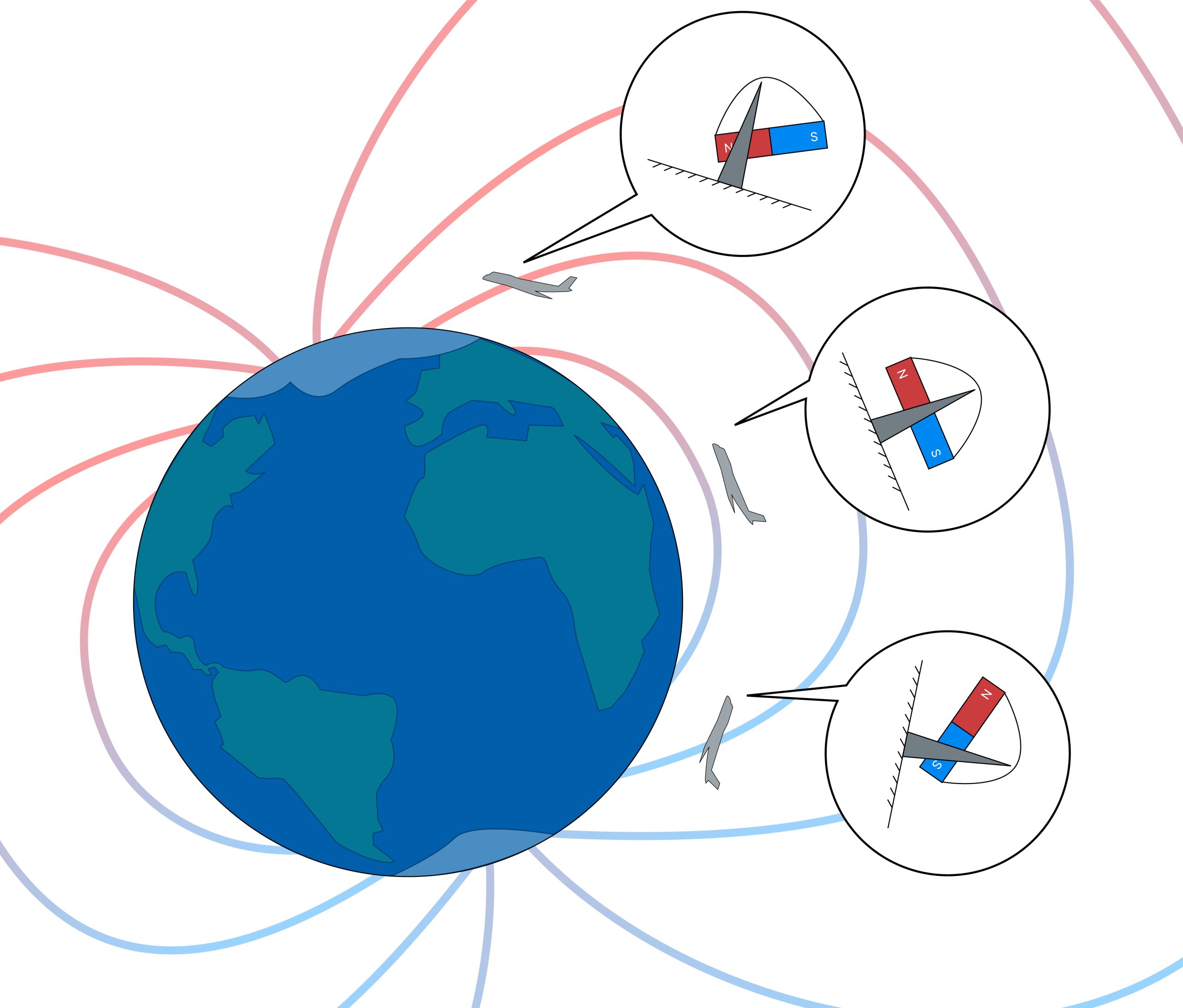
In a real navigational compass this is compensated by a system of bearings and counterweights to make sure that the needle actually floats horizontally and points toward north. However, in principle, we can use that inclination to measure latitude. Inclination and latitude are related trigonometrically by the formula
tan(I) = 2 tan(λ)
….where I = inclination and λ = latitude
We don’t normally do this with a navigational compass, because we have other ways of measuring latitude. However, this property becomes very useful in paleomagnetism, because certain kinds of rock, when they form, make a record of the earth magnetic field as it existed at the time of their formation. We call this remanent magnetism.
Remanent magnetism is particularly characteristic of rocks containing the mineral magnetite (Fe3O4), an iron oxide mineral that is commone (for example) in mafic igneous rocks like basalt. When basalt is first erupted, magnetite is too hot to retain a magnetic field, but as it cools through a temperature of about 570°C, known as the Curie point or temperature, it “locks in” the Earth’s magnetic field as remanent magnetization. If we are able to measure the declination and inclination of this “fossil” magnetic field, we can determine both the direction and the distance of the North or South Pole at the time the rock cooled through the Curie temperature.
Apparent polar wander paths
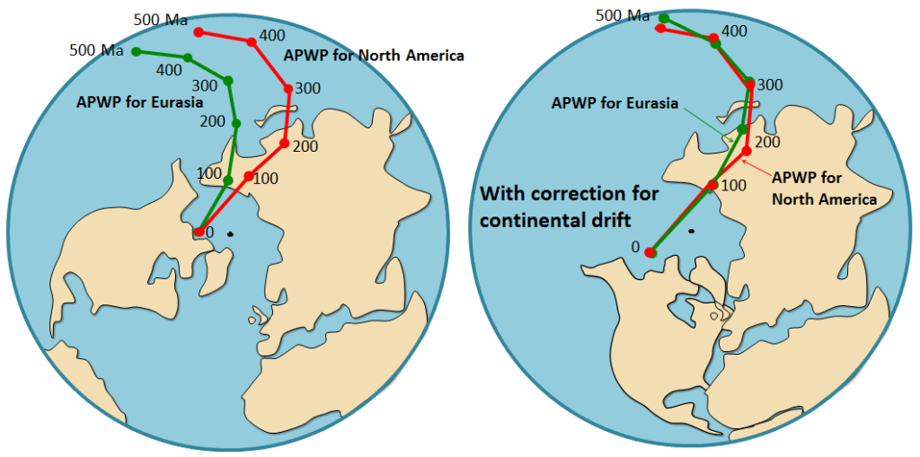
If we have a variety of suitable rocks from a particular region, we may be able to use measurements of remanent magnetism to determine the distance and direction of the pole at different times in geologic history. What we typically find is that the pole appears to have wandered over the Earth’s surface through time. We can therefore plot an apparent polar wander path or APWP. This tells us that one of two things must have occurred.
Either
- The pole wandered over the surface of the Earth; or
- The pole remained fixed but the continent drifted.
To distinguish these two options, we plot the APWP for two or more continents. If the pole moved, the APWPs should be identical. In fact, the APWPs turn out to be different for different continents, and they can only be superimposed if the positions of the continents are adjusted for movement across the surface of the Earth, as shown in the diagram.
During the 1950s, a majority of paleomagnetic specialists came to believe that the continents had indeed moved around. However, it took a second type of evidence to convince a majority of other Earth scientists.
Magnetic reversals
As increasing amounts of work were done on paleomagnetism in the 20th century, some puzzles emerged. In some cases, samples analysed for paleomagnetism gave results that were entirely consistent with nearby samples except that the polarity was reversed. Where a north pole was expected, a south pole was found, and vice versa. The idea arose that perhaps the remanent magnetism spontaneously reversed its direction. However, this became unlikely when isotopic dating was used to find the ages of samples, and it was found that there were some intervals of geologic time when all the samples gave reversed polarity. and others when normal polarity was consistently recorded. Hence, it had to be that the Earth’s magnetic field underwent a ‘flip’, reversing its polarity in a relatively short time. Although this hypothesis seemed outlandish when it was proposed, it’s now known that spontaneous magnetic reversals can occur when a magnetic dynamo operates in a liquid conductor like the Earth’s core, and the process has even been simulated using computer models.
As a result, it has been possible to build up a timescale of magnetic reversals going back to about 150 Ma. Reversals seem to occur haphazardly, every few hundred thousand years, but there have been intervals of time with very few reversals, when the Earth’s magnetic field has remained in the same polarity for millions of years. Not much is directly known about the process of reversal except that the time scale is quick (perhaps only a few hundred years). It seems that the magnetic field decays over time and breaks down into a weak field with a complex pattern of N and S poles (a non-dipole field), before rising back to its former strength, either with reversed polarity or with the same polarity as before.

About the same time, magnetic surveys were carried out from ships travelling in the oceans. These began to record patterns of magnetic anomalies – regions in which the Earth’s magnetic field is slightly stronger or weaker than would be predicted from the simple “bar-magnet” model of the magnetic field. In particular, when surveys were carried out across a mid-ocean ridge like the Reykjanes ridge south of Iceland, it was found that the ridge crest was always characterized by a strong positive anomaly, and that the pattern of negative and positive anomalies (sometimes called magnetic stripes) was symmetrical on either side of the ridge.
How could these curious patterns be explained? One phenomenon that can produce a magnetic anomaly is a body of rock with strong remanent magnetism. If the remanent magnetism is aligned parallel to Earth’s field, the two fields add to one another, and a positive anomaly will result. However, if the remanent magnetism records a reversed field, then it will subtract from the overall Earth’s field and a negative anomally will be recorded.
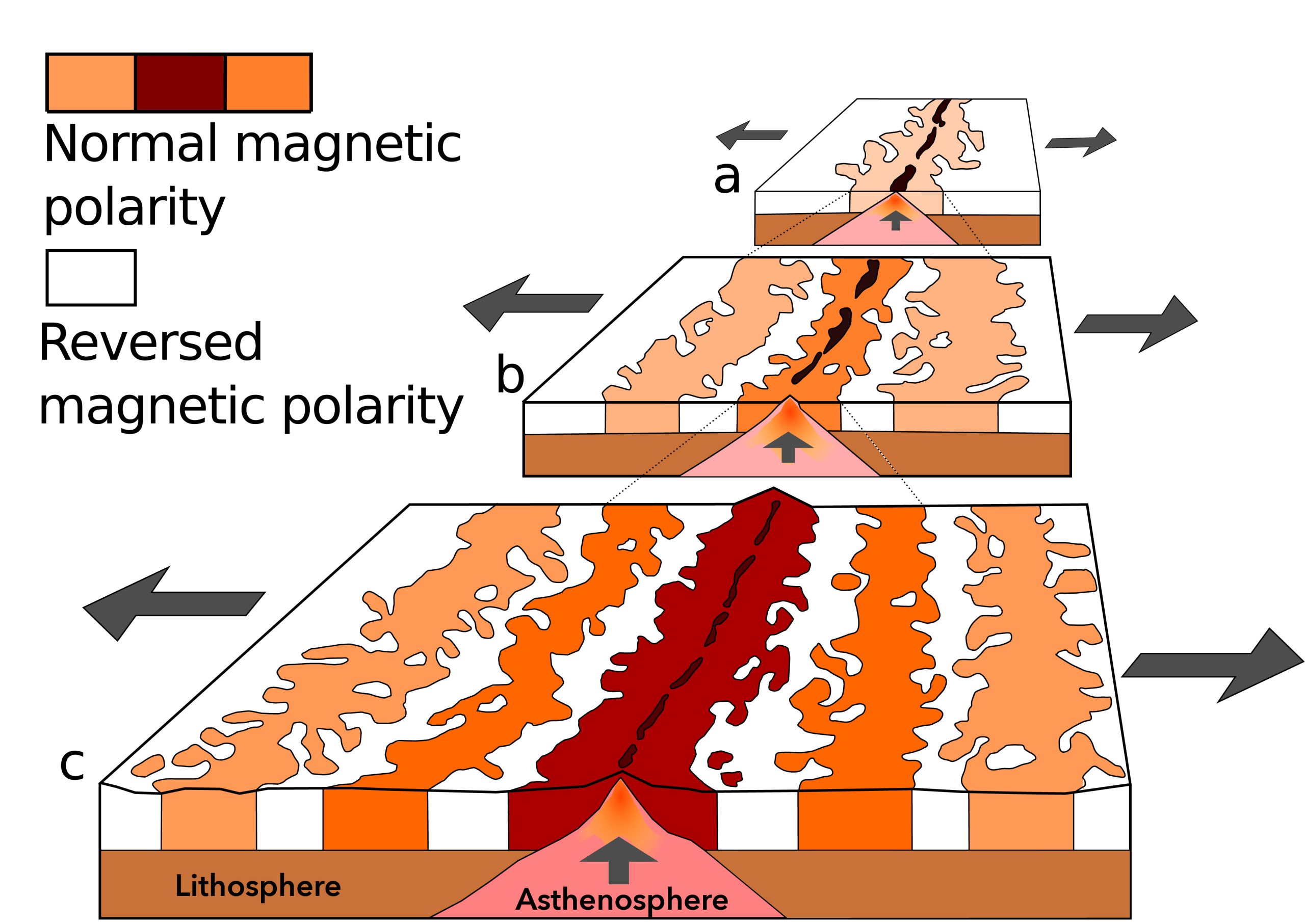
A number of geophysicists proposed an explanation. If new ocean floor is continuously forming, cooling, and spreading apart at the mid-ocean ridges, while the Earth’s core is undergoing reversals, the new ocean floor will effectively contain two recordings of the magnetic reversal history, recordings closely analogous to old-fashioned analogue magnetic tape recordings that were used to record music before the advent of digital media. Where the ocean floor contains normally magnetized basalt, a positive anomaly is recorded; where the ocean floor is reversely magnetized, the anomaly will be negative. The first scientist to propose this hypothesis was probably the Canadian geophysicist Lawrence Morley. However, his paper was rejected by the journal Nature as too speculative. A few months later, British graduate student Fred Vine and his supervisor Drummond Matthews independently came up with the same idea, but this time they had newly collected data to support it, and their paper was accepted in 1963. The idea that the pattern of magnetic anomalies in the oceans can be explained by a combination of ocean-floor spreading and magnetic reversals is commonly known as the Vine-Matthews-Morley hypothesis and paved the way for the modern theory of plate tectonics.
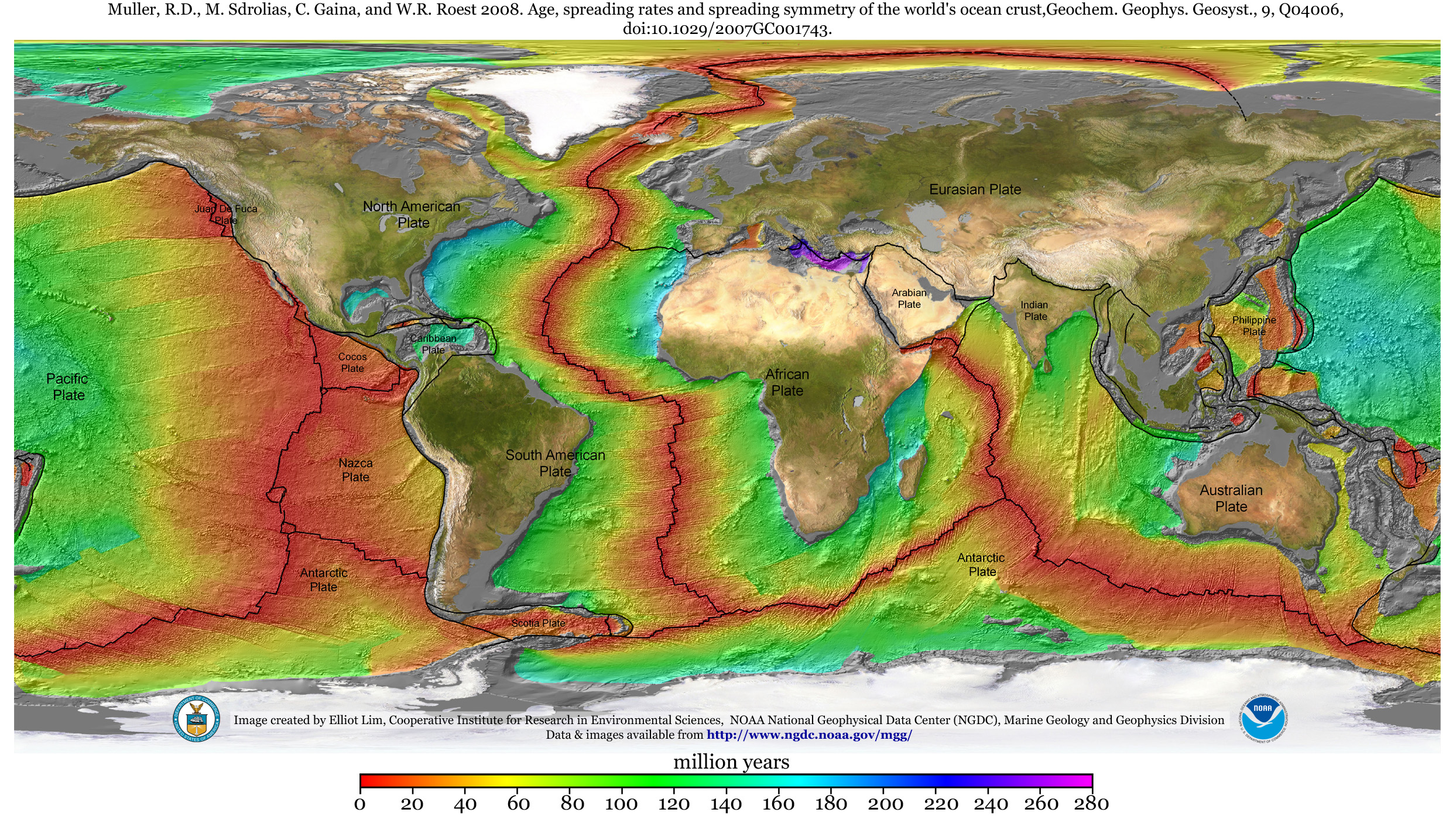
The pattern of magnetic reversals effectively provides a “bar code” for the age of the ocean floor. Using this bar code, geophysicists have been able to map the age of most of the Earth’s deep ocean floor. Surprisingly, the oldest ocean floor goes back only to about 200 Ma, in the early Mesozoic Era, showing that all the current ocean floors have formed in the last 5% of Earth history. In contrast, parts of the Earth’s continental crust are as old as 4 Ga, as shown by uranium-lead dating of zircon. Hence, unless the Earth has expanded suddenly and rapidly since 200 Ma (for which there is little evidence), the ocean floors must be continuously recycled into the mantle to make room for the new ocean floor formed at the ridges. This requires a “sink” for the ocean floor. The location of this “sink” depended on seismic data, which we will look at in the next section.
Seismicity
Earthquakes have been known from ancient times. They are known as seismic events and the geophysicists who study them are known as seismologists.
Earthquakes are very destructive envents and cause great loss of life, injury, and damage to property when they affect populated areas. It’s easy to think of them as rare and catastrophic events. However, earthquakes occur every day, and the seismic waves they produce can travel through the solid Earth, so they are able to provide information about the interior of the Geosphere that is very useful to Earth scientists. The major divisions of the Geosphere that we have met in other sections: the core, the mantle, and the crust, and the lithosphere and asthenosphere, were all discovered as a result of the study of seismic waves.
How earthquakes occur
Earthquakes occur at faults, brittle fractures or breaks in the rocks of the Earth’s upper layers. The basic process that causes earthquakes is relatively well understood, although that definitely does not mean that they can be predicted. Seismology is able to asses earthquake risk – the chance that an earthquake of a given magnitude will occur in a given area during a given time interval – but not the timing of individual events.
Earthquake risk results from the strain (change of shape or volume) of the rocks in a localized part of the Geosphere, typically in response to the movement of plates (although earthquakes can occur for other reasons). As the rocks distort, the differential stress within them rises proportionally. This type of deformation, where stress and strain are proportional, is known as elastic deformation. It’s the same type of behaviour that occurs in a spring or a car tire (although in rocks a much smaller amount of strain is associated with a given stress, because rocks are mostly much stronger that springs or tires). Typically rocks become distorted over periods of decades or centuries as the stress rises. Plate movement is typically measured in centimetres per year, and the strain may be spread over an area many kilometres wide. Within this region, energy is stored in the distorted rocks.
Eventually, the stress on some surface (often, but not always, a pre-existing crack) exceeds the frictional resistance along that surface, and slip occurs, starting an earthquake. In contrast to the long buildup, slip is extremely fast: once failure has occured, the rocks on either side of the fracture surface may move at speeds up to a few kilometres per second. Slip spreads rapidly over the fault surface: in a typical earthquake, a fault surface may slip, over a region, known as a rupture, that is kilometres to hundreds of kilometres wide. Whereas it may take decades to centuries for strain to build up, that strain is released in a period that lasts from a few seconds up to about 5 minutes for the largest earthquakes.
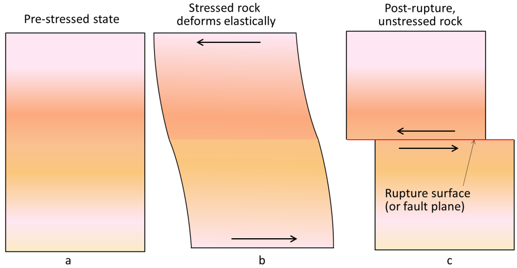
During an earthquake. the rocks on either side of the fault surface spring back rapidly to their unstrained shape, and the energy that was stored within them is released as vibrations, called seismic waves, that spread outwards from the slipped region in all directions. Depending on the type of earthquake, the ground in the vicinity of the earthquake may move up, down, or horizontally. Depending on the size of the earthquake, this motion may range from metres to a few tens of metres. By comparing accurate GPS (global positioning system) measurements before and after an earthquake, it’s now possible to measure this movement.
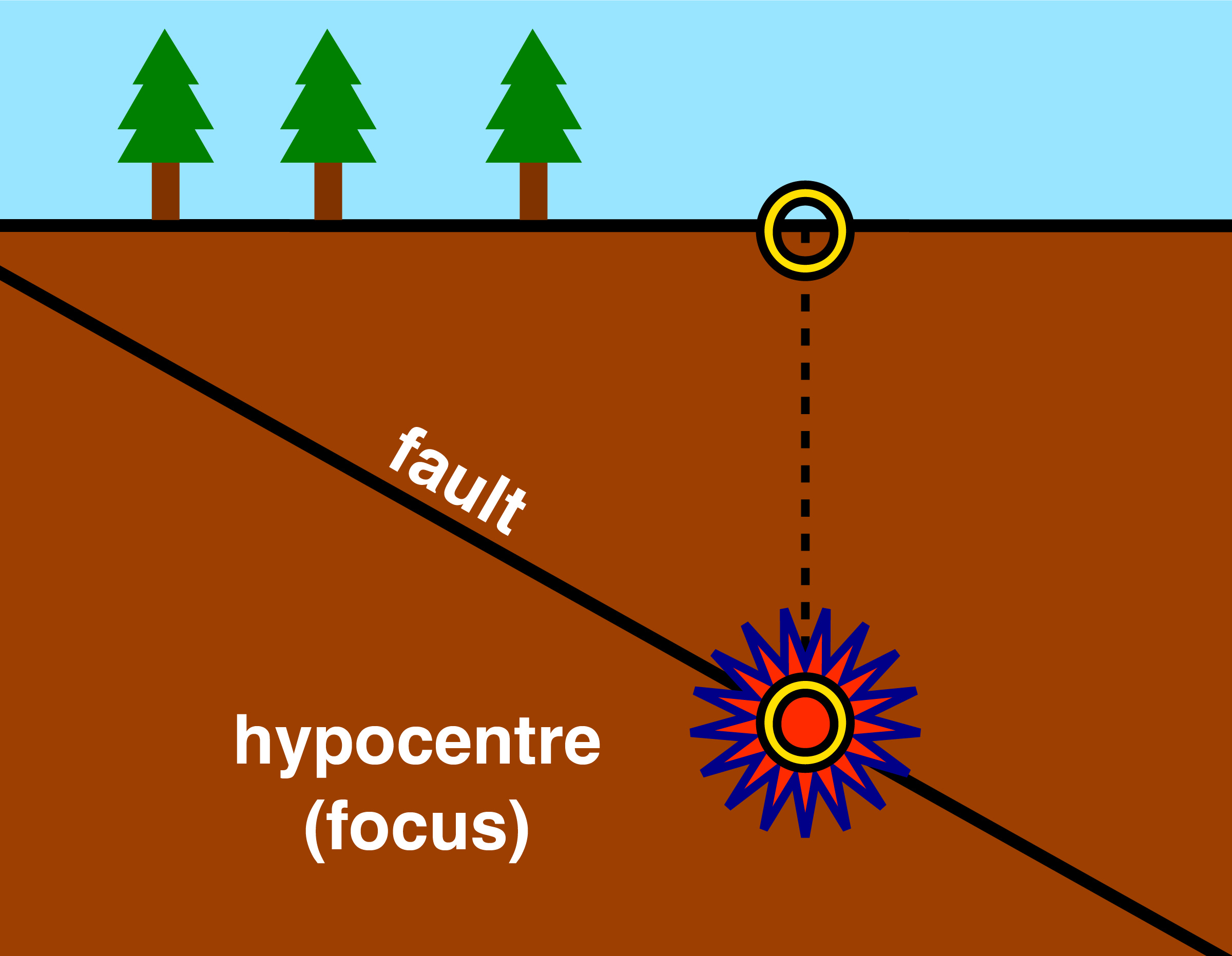
The point within the Geosphere from which the seismic waves originate is known as the focus or hypocentre of the earthquake. The depths of earthquake hypocentres (or foci) are quite variable: the deepest occur about 650 km below the surface. A point on the Earth’s surface directly above the hypocentre is called the epicentre. Note that the epicentre of an earthquake is at the surface of the Geosphere by definition. It’s common for news media to report the “depth” of an epicentre but this is quite wrong. They usually mean the hypocentre or focus!
Earthquake magnitude and intensity
Much of our knowledge of what goes on in an earthquake comes from observations of seismic waves by seismographs or seismometers that record the vibrations at a particular point on or within the Earth. Seismological web sites provide automated display of data when a major earthquake occurs anywhere in the world, often within minutes to hours after an event. A particularly thorough compilation can be found at
https://earthquake.usgs.gov
We can use these observations to compare the sizes of different earthquakes. There are two ways of doing this.
Earthquake intensity
The intensity of an earthquake is a measure of the ground shaking at a particular point. Its measured with a device called a seismograph or seismometer. Typically, this device has a suspended weight that has inertia, causing it to stay still during an earthquake, while a recording device beside it is fixed to the earth, which moves around as the earthquake passes. Early seismographs recorded this movement mechanically, with a moving pen dragging across paper, but all modern seismometers operate with electronic sensors.


Intensity is one of the most important variables for measuring the destructive potential of an earthquake. There are a number of ways of measuring intensity. One of these is the modified Mercalli scale (named after the Italian seismologist who devised it). In this scale, a value of I is assigned to shaking that is imperceptible except to seismographs, while intensity II describes an earthquake that is noticed only by people sitting or lying still. At the other extreme, an intensity of XII describes seismic vibrations that cause total destruction of buildings and throw objects into the air.
| Intensity | Acceleration (% g) | Shaking | Damage |
| I | <0.046 | Weak | Recorded only by seismographs |
| II | 0.046–0.3 | Weak | Persons at rest |
| III | 0.3–1.1 | Weak | Persons indoors |
| IV | 1.1–2.8 | Light | Felt by many; windows rattle |
| V | 2.8–11.5 | Moderate | Felt by most; some dishes, windows break |
| VI | 11.5–21.5 | Strong | Felt by all; furniture moved; rare building damage |
| VII | 21.5–40.1 | Very strong | Slight to moderate building damage |
| VIII | 40.1–74.7 | Severe | Damage, partial collapse of buildings; furniture overturned |
| IX | 74.7–139 | Violent | Much building damage; Buildings moved off foundations |
| X | >139 | Extreme | Most buildings damaged; bridges twisted |
| XI | Extreme | Most buildings collapse | |
| XII | Extreme | Total damage; waves seen on ground surface; objects thrown into air |
Another way of measuring intensity is by ground acceleration. That acceleration may be compared with the acceleration due to gravity, g, equal to 9.81 m/s2. For objects to be thrown into the air (in the most catastrophic earthquakes), the vertical ground acceleration must exceed 100% of the acceleration due to gravity.
Intensity measures the strength of an earthquake at a particular point, so it’s an intensive variable. Intensity is only loosely correlated with the total energy released in an earthquake (its magnitude). Intensity does depend on this total energy, but it also depends on the distance of the measurement from the earthquake focus, and also on the susceptibility of particular rocks or sediments to shaking.
Earthquake magnitude
Earthquake magnitude is an extensive variable that measures the total energy release of a seismic event. The American seismologist Charles Richter first developed a scale of earthquake magnitude by measuring the maximum amplitude (i.e. distance) of ground shaking, a measure of intensity, at a standardized distance from the earthquake focus. To cover the huge range of intensities observed, the Richter magnitude scale is logarithmic, so that a magnitude 7 earthquake produces ground motion that is ten times larger than a magnitude 6 earthquake, and 100 times larger than one with magnitude 5. Because of the complex way in which ground shaking is related to stored energy, the each step on the magnitude scale increases the energy released by a factor of the square root of 1000 or 31.6. A magnitude 6 event is 31.6 times as energetic as a magnitude 5 event; a magnitude 7 event releases 1000 times as much energy as a magnitude 5 event.
It turns out that maximum amplitude is not a very good measure of energy output for very large earthquakes, nor for very small ones. More sophisticated measures of energy release have largely replaced Richter’s method. Most modern estimates use a moment magnitude (Mw) scale that has been calibrated so that the numbers roughly match Richter’s for moderate earthquakes (magnitude 6). Media reports typically refer to these values as “on the Richter scale” although this is not technically correct.
| Magnitude | Energy (joules) | Equivalent TNT explosion (tonnes) | Descriptor | Number annually |
| 1.0–1.9 | >1.3 x 10⁸ | Micro- | ||
| 2.0–2.9 | >4 x 10¹⁵ | Very minor | 1,300,000 | |
| 3.0–3.9 | >1.3 x 10¹¹ | >32 | Slight | 130,000 |
| 4.0–4.9 | >4 x 10¹⁵ | >1000 | Light | 13,000 |
| 5.0–5.9 | >1.3 x 10¹⁴ | >31,600 | Moderate | 1,300 |
| 6.0–6.9 | >4 x 10¹⁵ | >1,000,000 | Strong | 130 |
| 7.0–7.9 | >1.3 x 10¹⁷ | >31,600,000 | Major | 17 |
| 8.0–8.9 | >4 x 10¹⁸ | >1,000,000,000 | Great | 1 |
| >9.0 | >1.3 x 10²⁰ | >31,600,000,000 | Extreme | <1 |
Earthquakes with moment magnitudes above 8 are referred to as “great” earthquakes. They occur at a frequency of about one per year, on average. Exceptional earthquakes have magnitudes over 9; these occur only a few times per century; only five have been recorded in the 70 years since accurate measurements became possible.
Seismic waves
When an earthquake occurs, seismic waves radiate out from the focus in all directions from the focus: north, south, east, west, up, and down, and all directions in between. These waves are known as body waves because they radiate through the interior (the ‘body’) of the geosphere. The upward-travelling waves hit the surface of the Geosphere around the epicentre, where some of their energy is transferred into surface waves, which spread out over the surface of the Geosphere or Hydrosphere like waves on the ocean. Body waves are most informative to geophysicists seeking information about what’s inside the Geosphere. Surface waves are the most damaging for Earth’s inhabitants.
Different types of seismic waves travel at different speeds, although these speeds are typically measured in kilometres per second, much faster than most of the processes we have examined in other parts of this course. Because they travel at different speeds, different types of seismic waves become more and more separated as they travel farther from an earthquake focus.
We will look at body waves and surface waves in turn.
Body waves
P-waves
P-waves are essentially the same as sound waves. They cause small vibrations in solid rocks which are directed towards and away from the earthquake focus, momentarily compressing and expanding the rock. They travel fast, arriving first at seismometers. Their full name is primary waves, because they arrive first at seismic stations. However, they can also be described as pressure waves or push-waves, words which more graphically describe their behaviour. For a precise definition we can say that P-waves are body waves in which the vibration direction is parallel to the propagation direction.
P-waves can travel through solids, liquids, and gases. In rocks of the Earth’s crust, they travel at speeds of 2–7 km/s, whereas in the mantle their speeds increase downwards, from 8 km/s at the top of the mantle to around 13 km/s at its base. P-waves, like all seismic waves, tend to travel slower in liquids and gases. The speed of P-waves (sound waves) in water is about 1.5 km/s, wheras in air it is only 0.34 km/s.
S-waves
S-waves are body waves in which the vibration direction is perpendicular to the propagation; that is to say, as the wave is moving forward, the atoms in the rock they pass through vibrate from side to side. S-waves travel slower that P-waves, lagging behind them and arriving second at seismometers that are distant from the focus; their name, short for secondary waves, derives from this timing. However, shear waves or shake waves are terms that also begin with “s” and help to describe their behaviour.
S waves travel at 1.5–5 km/s in the crust, and increase in speed to about 7 km/s in the lower parts of the mantle.
Unlike P-waves, S-waves cannot travel through fluids (liquids or gases) because fluids do not respond elastically to being sheared. This property of S-waves is one of the most important ways we can probe the interior of the Geosphere; it’s our main line of evidence that the mantle is solid whereas outer core is liquid, because S-waves cannot pass through it.
Surface waves
Rayleigh and Love waves
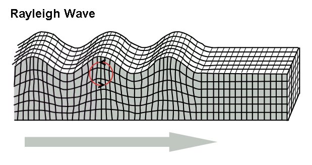
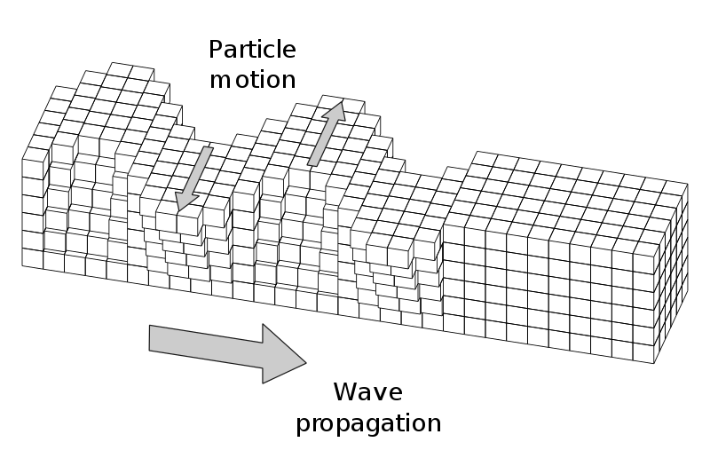
When P-waves and S-waves reach the surface of the Geosphere, part of their energy is transformed into surface waves: waves that bend the Earth’s surface rather like the waves on a pond when a rock is thrown into it. The surface waves radiate in expanding circles from the epicentre. These waves tend to have much higher amplitude than P-waves or S-waves, but they travel more slowly. Away from the epicentre they may arrive several seconds or minutes later than the S-waves. However, because of their high amplitude, they account for much of the destructive power of earthquakes. Two types are recognized, named after their discoverers.
Rayleigh waves are characterized by up-and-down movements of the Earth’s surface, although there’s also back-and-forth motion. Their behaviour is similar to waves on water, except that the direction of motion of the wave orbitals is in the opposite sense. In the highest intensity earthquakes, observers have been able to see Rayleigh waves rolling accross the land surface.
Love waves are a second type of surface waves characterized by horizontal, side-to-side shearing motion of the ground. These have no counterparts in the oceans, for the same reason that S-waves don’t travel through water: fluids have no elasticity when sheared.
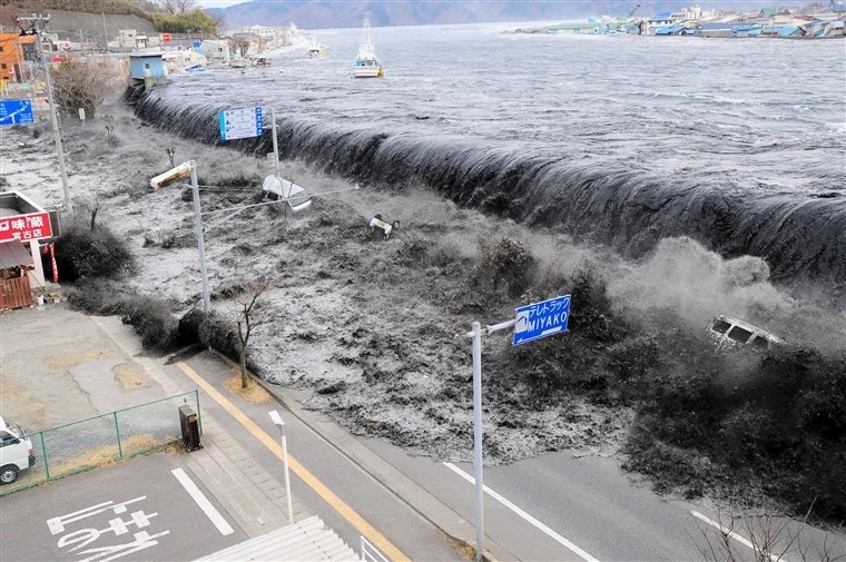
Tsunami waves
Surface waves also travel on the ocean. Such waves are very low on the open ocean (perhaps 1 m high). They travel slower than most other seismic waves (about 200 m/s) but still very fast (over 700 km/hr) compared with wind-driven waves. When they run into shallow water, they slow down and water can pile up to produce towering waves more than 10 m high. These waves can devastate coastal communities. Earthquake-generated waves were formerly known as ‘tidal waves’ but, because they have nothing to do with tides, the Japanese term tsunami is now used all over the world to describe earthquake-generated water waves.
Tsunami waves have been recorded in earthquake-prone Japan for centuries, and the relationship between earthquakes and tsunamis is well known. A tsunami recorded in Japan in 1700 CE was not matched with a nearby[2] earthquake and became known as the “orphan tsunami”. This tsunami probably originated on the opposite side of the Pacific Ocean where it devastated Indigenous communities as recounted by Chief Louis Clamhouse[3]:
“This story is about the first !Anaqtl’a or “Pachena Bay” people. It is said that they were a big band at the time of him whose name was Hayoqwis?is, ‘Ten-On-Head-On-Beach.’ He was the Chief; he was of the Pachena Bay tribe; he owned the Pachena Bay country. Their village site was Loht’a; they of Loht ‘a live there. I think they numbered over a hundred persons…. There is no one left alive due to what this land does at times. They had practically no way or time to try to save themselves. I think it was at nighttime that the land shook … They were at Loht ‘a; and they simply had no time to get hold of canoes, no time to get awake. They sank at once, were all drowned; not one survived … I think a big wave smashed into the beach. The Pachena Bay people were lost…But they on their part who lived at Ma:lts’a:s, ‘House-Up-Against-Hill ‘, the wave did not reach because they were on high ground. Right against a cliff were the houses on high ground at M’a:lsit, ‘Coldwater Pool’. Because of that they came out alive. They did not drift out to sea along with the others…”
Finding the location of an earthquake
Because P-waves travel faster than S-waves, the two waves get farther and farther apart as they travel through the Earth. The time interval between the arrival of the first P-waves and the first S-waves can be used to calculate a distance to the earthquake focus, and ultimately to locate the earthquake.
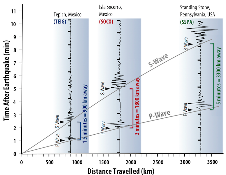
The graph shows the travel times of S-waves and P-waves, and the S-P delay (the time between the two arrivals) which increases with distance.
Suppose the P–S delay, for a shallow earthquake at a seismic station indicates a distance to the focus of 900 km. Then the focus must lie somewhere on a circle of radius 900 km centred on the station. If the same earthquake is picked up by a second station, and the P–S delay indicates a distance of 1800 km, then a larger circle can be drawn centred on the second station. The two circles will intersect at two points, possible locations of the earthquake. A third record of the earthquake is necessary to choose between these two points.
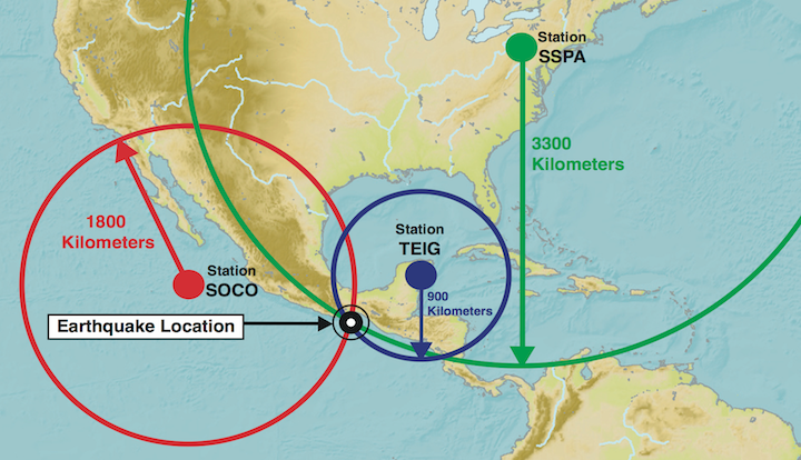
In the above example we have supposed that the earthquake is shallow, and therefore the focus is close to the epicentre. If we didn’t know the depth, then a fourth record from another seismometer would be sufficient to locate the focus in three dimensions.
In practice, large earthquakes are picked up by many more than four seismometers worldwide, so multiple distances are calculated and the published location of the earthquake is a best fit to all the available data.
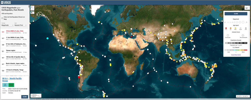
Locations of earthquakes are posted, soon after they occur, at https://earthquake.usgs.gov
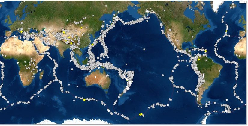
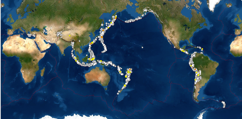
When depths are plotted on a map, it becomes apparent that the vast majority are shallow-focus earthquakes, with depths less than 30 km. However, in certain parts of the world, intermediate-focus (70–300 km) and deep-focus earthquakes (300–700 km) occur. Most of these locations are close to the deep ocean trenches.
Earthquakes and the interior of the Geosphere
Seismic waves are able to pass right through the Geosphere. When a large earthquake occurs, it’s common for the seismic waves to be detected on the opposite side of the Earth, arriving a little over 20 minutes later. On their way through the Earth, sesimic waves pass through the crust, mantle and core, and within the mantle, they pass through the most plastic part of the mantle, the asthenosphere, and the more rigid parts above and below (the lithospheric upper mantle, and the lower mantle). Seismic waves therefore can be used to probe these internal parts of the Earth, which are far beyond the reach of drilling. (The maximum depth to which humans have drilled in 2023 is a little over 12 km.)
Behaviour of seismic waves
The behaviour of seismic waves is in many ways like that of light waves, enabling us to “see” into the otherwise opaque interior of the geosphere. Diagrams showing the full pattern of waves can be quite complex, so it’s often easier to show rays, paths that show the direction of travel of the seismic energy. Rays and waves are closely related: the rays are oriented perpendicular (at 90°) to the waves themselves.
Reflection
When seismic waves encounter a boundary between different rock types, they may bounce off the boundary process, a process known as seismic reflection. Reflection can occur wherever there is a change in acoustic impedance (density multiplied by the velocity of seismic waves in the material). Within the crust, reflections of seismic waves are used in exploration for resources. The reflection of seismic waves follows the same laws as the reflection of light from a mirror: the angle that the reflected waves make with the reflection surface is the same as the angle of the incoming waves. Within the Earth as a whole, reflections most prominently occur at the core–mantle boundary.

Refraction
Seismic waves undergo refraction wherever there is a change in seismic velocity, the speed of the seismic waves, from one material to another. Seismic waves approaching the boundary “head on” are unaffected by refraction, but the path of any seismic waves that approach the boundary at an angle is changed. In general, the direction of travel of the waves is bent towards the boundary in whichever rock type has the higher velocity, and away from the boundary in the material with the lower velocity.
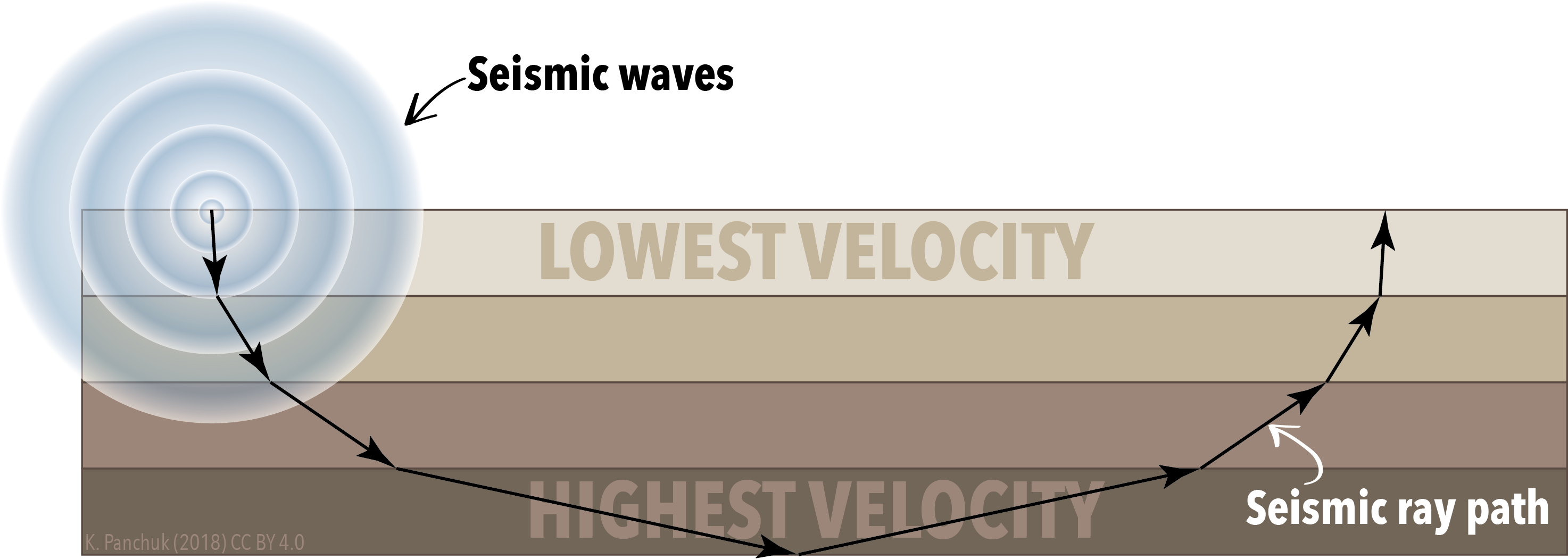
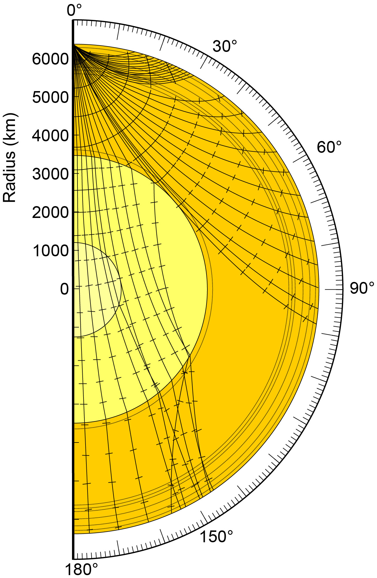
Because the velocity of seismic waves in the mantle typically increases downward, the direction of travel of diving seismic waves becomes flatter and flatter with depth, such that some can actually be refracted back up towards the surface.
Attenuation
Seismic waves are also absorbed by some types of Earth materials. Partially molten rock, such as occurs in the asthenosphere is quite effective at absorbing and slowing down seimic waves. The asthenosphere was first detected as a result of the attenuation and retardation (slowing down) of seismic waves passing through it. Another example is the Earth’s outer core, which is completely liquid. Because of this it is completely unable to transmit seismic S-waves.

Internal divisions of the Geosphere
Moho
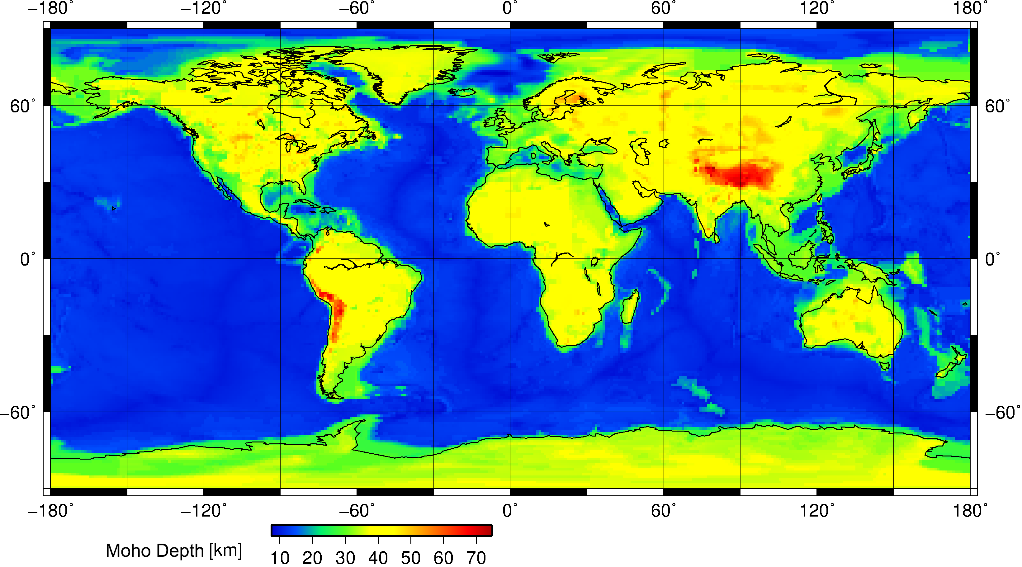
One of the earliest divisions to be identified within the Earth is named after the Croatian seismologist Andrija Mohorovičić. The full name of the feature is the Mohorovičić discontinuity but it is most often referred to simply as the Moho. At the Moho, P-waves are sharply refracted because their velocity increases abruptly from values below about 7 Km/s to above 8 km/s. The Moho typically lies at depths 5–10 km below the ocean floor, but 20–90 km (typically 30–40 km) below the surface of continentals (including the continental shelves). The crust is defined as the part of the Geosphere that lies above the Moho. In some ways, this definition is unfortunate; it was established well before the theory of plate tectonics and before the asthenosphere was identified. Because the word ‘crust’ conjours up a picture of something rigid, many assume that tectonic plates are made of crust. In fact we now understand that the most rigid part of most plates is the lithospheric upper mantle; parts of the crust are actually weaker than this strong, lower part of a plate. Remember that plates are made of lithosphere and that crust is only the upper part of each plate.
The properties of the rocks below the Moho, deduced from gravity and seismic data, correspond to peridotite: an ultramafic rock composed largely of ferro-magnesian silicate minerals, mainly olivine. The rocks above the moho, are much more varied. Where the crust is oceanic, it mostly comprises mafic igneous rock, containing feldspar and ferromagnesian minerals. The continents are much more varied, comprising all the rock types described in the rock cycle. Many of these also contain minerals of the framework-silicate feldspar group, and quartz is abundant. To a first approximation the Moho can be viewed as a boundary between rocks with little or no feldspar (below) and rocks with abundant feldspar (above).

Low velocity zone (Asthenosphere)
Farther down within the mantle, starting typically about 100 km below the Earth’s surface, is a low-velocity zone where the velocity of both P and S-waves declines slightly, and where S-waves are slightly attenuated, suggesting that there is a small amount of liquid. Mantle rocks are probably slightly above their solidus temperature, so there may be about 5% melt present in this zone, known as the asthenosphere. The base of the asthenosphere is rather poorly defined: the peridotite of the upper mantle becomes more solid both downward (due to higher pressure, which raises the melting point, and due to the development of new minerals) between about 250 and 650 km.
Outer core
The core-mantle boundary, about 2900 km below the surface, is the most abrupt and major change in properties within the Earth. P-waves are dramatically slowed down, and as a result, incoming P-waves are refracted downward, toward the centre of the Earth, if they arrive obliquely at this boundary. They are also partially reflected back towards the Earth’s surface. Because of its lower P-wave velocity, the core acts like a lens, focusing the P-waves into a smaller area on the opposite side of the Earth from the epicentre, and leaving a ring-shaped P-wave shadow zone where no P-waves are recorded by seismometers between about 11,500 and 16,500 km from the epicentre. (Between 104° and 148° measured as an angle around the Earth.)

S-waves are completely blocked by the core, so very little S-wave energy is received beyond 11,500 km from the epicentre. The S-wave shadow zone is therefore a large circular area including everything beyond 104° from the epicentre. (A very small amount of S-wave energy is re-generated as P-waves escape from the core.)
Inner core
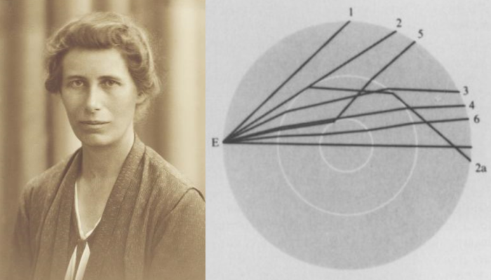
The inner core was discovered by Danish geophysicist Inge Lehman, studying earthquakes with epicentres in New Zealand, recorded by seismometers on the opposite side of the Earth. In the central part of this region, p-waves arrive slightly earlier than elsewhere, indicating that they have been accelerated, but only if they pass within about 1200 km of the centre of the Earth. Some recording sites receiv two closely spaced arrivals of p-waves, a first arrival that has travelled through the inner core, and a second arrival that has travelled a little more slowly through the liquid outer core. From these timings of p-wave arrivals, it was deduced that there must be a seismically faster, probably solid body at the centre of the core. It is suspected that the inner core has slowly grown, as the Earth has cooled through geologic time, and molten iron has gradually frozen on to the inner core.
Interestingly, inside Mars, the metallic core is solid at the present day. As a result, the magnetic field of Mars is much weaker than that of the Earth. However, strong remanent magnetism has been detected in ancient rocks on Mars by orbiting artificial satellites. Hence, Mars must have had a liquid outer core, like Earth’s, that eventually entirely solidified as the solid inner core grew.
Plate tectonics
Plate boundaries
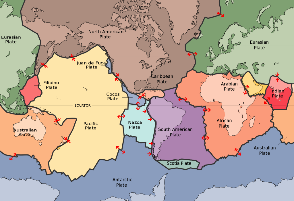
When earthquake epicentres are plotted on a map of the Geosphere, it becomes clear that their distribution is not random. For example, each of the mid-ocean ridges identified as a centre of sea-floor spreading is marked by a line of epicentres. In addition, if we look only at intermediate-focus and deep-focus earthquakes, these are concentrated below the deep ocean trenches. Using information from earthquakes, in conjunction with data from magnetic anomalies, it is possible to join these linear zones up into a network of plate boundaries. These plate boundaries separate tectonic plates, pieces of the lithosphere, which is able to slide slowly over the asthenosphere below.
It’s important to note that the lithosphere, typically about 100 km thick, comprises both the crust and the upper part of the mantle, known as the lithospheric upper mantle. Most plates contain portions with both continental and oceanic crust.
Plate boundaries are of three types, depending on whether the plates are moving apart, sliding past each other, moving towards one another. We will look at each type of boundary in turn.
Spreading centres
Spreading centres, or divergent plate boundaries typically occur at mid-ocean ridges. We have already met the spreading centres in the section on linear magnetic anomalies. Along these boundaries, two plates are moving apart, and hot, plastic mantle from the asthenosphere rises to fill the space between them. The mantle rises adiabatically, and as explained in the section on igneous rocks the release of pressure causes it to undergo partial melting, producing mafic magma. This magma rises toward the surface and solidifies at the mid-ocean ridge, forming new oceanic crust, mostly made of mafic igneous rock, continuously filling the ‘gap’ that would otherwise arise between the two plates, and adding material to the two plates.
The earthquakes that occur at spreading centres are shallow, typically between 0 and 30 km depth. Below this, the rocks are probably too hot to undergo the brittle fracture behaviour that is necessary to produce earthquakes.
The residual (leftover) mantle that remains after partial melting also becomes more solid, once the melt has been extracted. It forms the lithospheric upper mantle, the majority of the plate.
Ocean-floor spreading is typically roughly symmetrical: in other words, the plates on either side grow at about the same rate, resulting in the symmetrical patterns of magnetic anomalies that are typically seen. The Mid-Atlantic Ridge and the East Pacific Rise are good examples.
Transform faults
Many of the mid-ocean ridges show small right-angle (90°) offsets that mark places where the plates slide past one another rather than being pulled directly apart. Plate boundaries like this, where relative plate motion is parallel to the boundary, are called transform faults. We can recognize two types of transform fault, depending on the sense of motion.
If an observer stands on one side of a transform fault, and when looking towards the opposite side, sees the opposite side moving to the right, the fault is dextral, or right-lateral. Another way to think about this is to imagine a ball-bearing caught up and rolling in the fault zone. The rotation of the ball-bearing is clockwise.
If an observer stands on one side of a transform fault, and when looking towards the opposite side, sees the opposite side moving to the left, the fault is sinistral, or left-lateral. Another way to think about this is to imagine a ball-bearing caught up and rolling in the fault zone. The rotation of the ball-bearing is counterclockwise.
Not all transform faults are like the short segments that connect parts of the mid-ocean ridges. Others are much longer, extending for hundreds or thousands of kilometres before connecting with other types of plate boundary. The most famous example is the San Andreas Fault, that separates the Pacific Plate from the North American Plate, with continental lithosphere on both sides.
Earthquakes at transform faults are almost always shallow. Because the crust is not as hot as at mid-ocean ridges, earthquakes are actually more frequent on transform faults than on the ridge segments at a typical mid-ocean ridge.
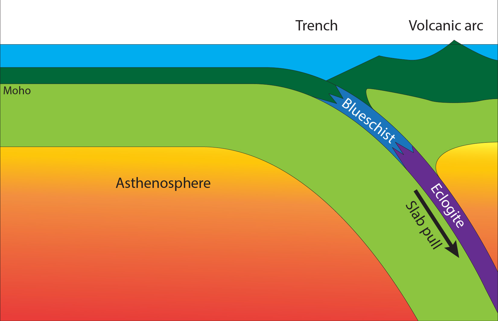
Subduction zones
A third type of plate boundary occurs where plates are converging. Typically, convergence is highly asymmetric and one plate dives beneath the other. The diving lower plate is said to be subducted beneath the upper plate. Above the subducted plate, there is typically a deep-ocean trench which is typically accompanied by a negative gravity anomaly, showing that the lithosphere is not in isostatic equilibrium. Something is pulling it down.
Boundaries of this type are known as subduction zones, trenches, or simply as convergent plate boundaries.
On the upper plate, there is, in many cases a chain of volcanoes called a volcanic arc. Most typically, these erupt intermediate magma, producing spectacular conical volcanoes like Mount Fuji in Japan or Mount Ranier in Washington state.
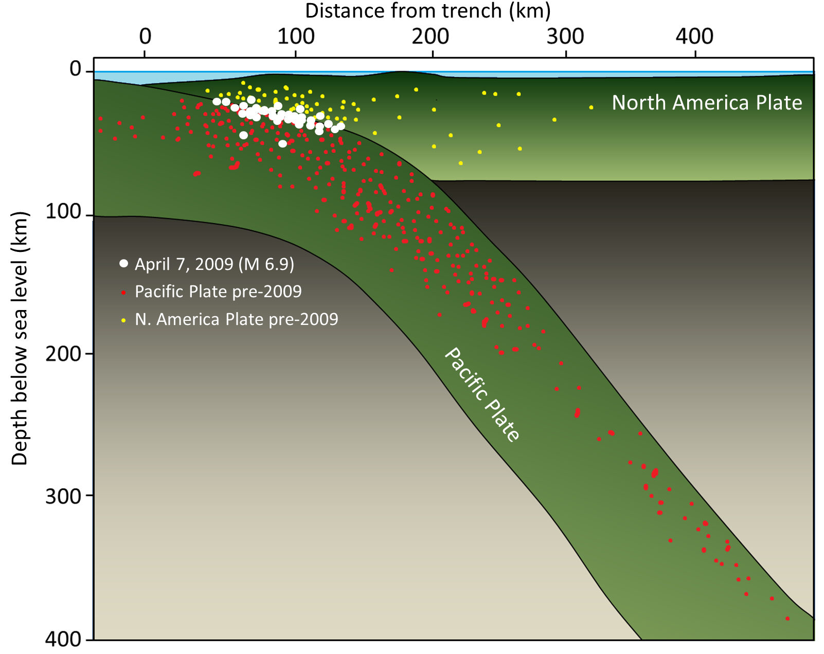
The Earth’s intermediate to deep-focus earthquakes occur in subduction zones. In many cases there is a sloping zone of earthquake hypocentres beneath the upper plate that deepens away from the plate boundary. This zone is known as the Wadati-Benioff Zone, or just Benioff Zone, after the geophysicists who discovered it. It is believed to mark a slab of the lithosphere of the subducted plate as it descends within the mantle. The rocks of the subducted plate take millions of years to warm up to the temperature of the surrounding mantle. Because they are cold, they can undergo brittle fractures at depths much greater (down to 650 or 700 km) than those that characterize other types of plate boundary.
Most of the deep ocean trenches around the Pacific Ocean (the “ring of fire”) mark subduction zones. Examples include the Peru-Chile trench off the coast of South America and Mariana Trench in the west Pacific. Note that in a subduction zone the lower plate normally carries oceanic crust into the trench, but the upper plate, where the volcanic arc occurs, may be oceanic (as in the Mariana arc) or continental (as in the case of the Peru-Chile subduction zone).
Direct measurement of plate motion
GPS
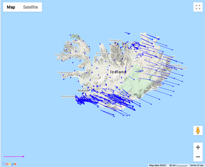
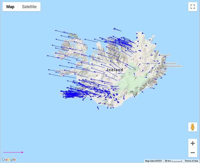
Although the theory of plate tectonics was developed largely on the basis of seismic and magnetic data, it has become possible since about the year 2000 CE to measure plate motion directly using the Global Positioning System (GPS). The rates of plate movement are slow: a few centimetres per year, so very precise GPS measurements are needed (much more precise than those made with consumer models). Typically, a measurement site must be occupied, or repeatedly visited with the same instrument, over a period of years, and careful averaging must be done to reduce the effects of random errors that occur at the limits of precision. Nonetheless there are now large numbers of measurements available and these can be accessed at a publicly available compilation site operated by the organization UNAVCO.
https://www.unavco.org/software/visualization/GPS-Velocity-Viewer/GPS-Velocity-Viewer.html
In interpreting data on plate motion it’s important to be aware of your frame of reference. The UNAVCO site allows users to pick any one plate as fixed and to view the motion of all the other plates relative to that one “fixed” plate. However, the choice of “fixed” plate is arbitrary, as all the plates move relative to one another. Our measurements from magnetic, seismic, and even GPS data tell us about relative movement between plates, but don’t give us an absolute frame of reference.
In addition, plate boundaries are are also in motion relative to one another. So, for example, the African plate is surrounded on three sides by spreading centres but it is not being compressed. The African plate is expanding, and as it expands the mid-ocean ridges that largely surround it are moving away from each other.
Hotspots
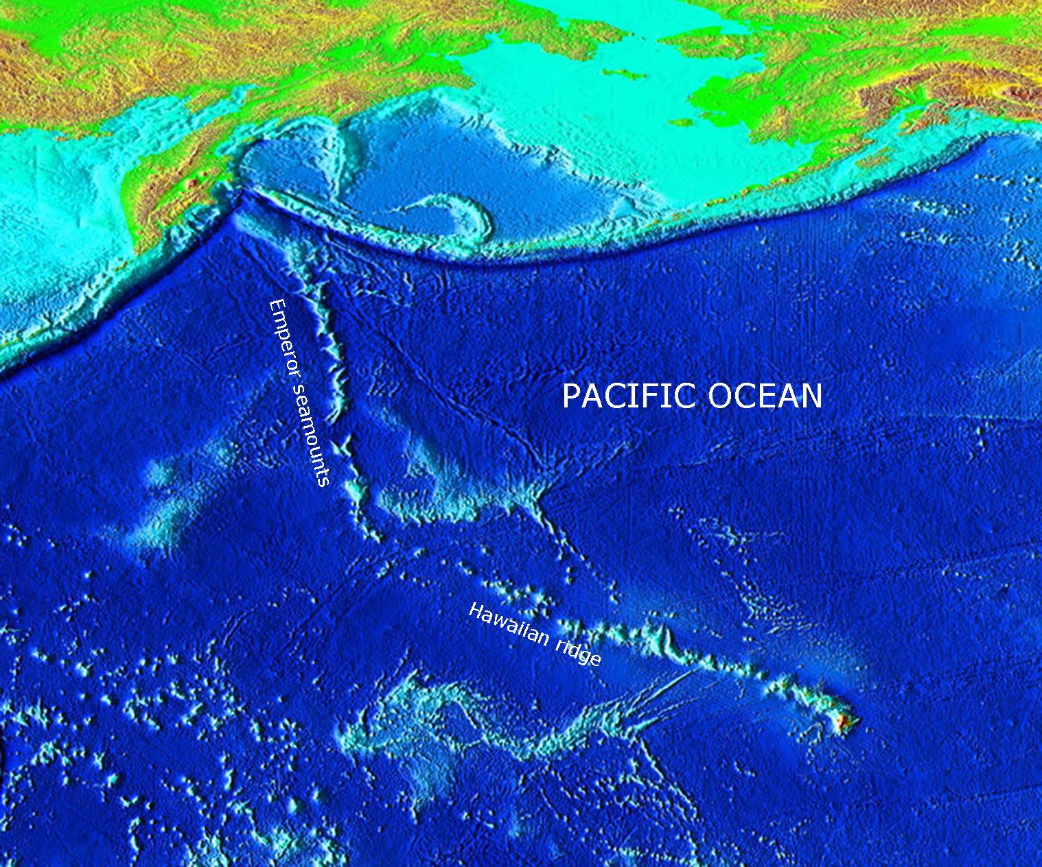
Not all volcanoes are found at plate boundaries. Some occur in the middle of plates. The best known example involves the island of Hawai’ia, which occurs in a group of islands (and archipelago) in the middle of the Pacific Plate. A chain of seamounts extends thousands of kilometres to the NW, and then to the N, starting at the Hawai’ian archipelago. These islands are all largely composed of mafic volcanic rock (basalt) derived by partial melting in the mantle. They formed as a result of the uprise of mantle material in a mantle plume, forming a hotspot in the Pacific Plate, feeding magma up to the seafloor. As the Pacific Plate moved, the volcanic islands were carried with it to the NW, and a new volcanic island formed a sort distance to the SE.

Isotopic dating shows that this movement has been going on since at least 59 Ma, early in the Cenozoic Era, and that there was a change in the direction of movement around 45 Ma. It’s easy to calculate the rate and direction of motion of the Pacific Plate relative to the hotspot, so this suggests a way of measuring absolute plate motion, relative to the underlying mantle. Unfortunately, when we try this with different hotspots, including those in the Atlantic and Indian oceans, we discover that the hotspots are moving relative to each other as well, although not as fast as the plates themselves. Therefore, even the hotspots don’t give us a perfect frame of reference within which to measure absolute plate movements.
Mechanism of plate motion
What drives the plates?
The only known energy source within the Geosphere is geothermal heat, and it has been estimated that about 1% of the Earth’s heatflow (about 0.4 of about 47 TW) is converted to mechanical energy by the processes of plate tectonics. The mechanism must be some form of convection, the process whereby hot material becomes less dense and therefore rises, while cold material is more dense and sinks. Convection is the process that keeps water moving in a boiling pot on a stove. However the process of plate tectonics is very different from a boiling pot of water, heated from below. The most rapid temperature change (the maximum temperature gradient) is at the top of the Geosphere, where the crust is rapidly cooled by conduction of heat into the hydrosphere and atmosphere. In addition, the tectonic system differs from a pot of boiling water in having a relatively rigid lid at its upper surface, the lithosphere.
Calculations on the forces acting on the plates suggest that two large forces are most important. The largest is what is known as the slab pull force. As the lithosphere enters a subduction zone, mafic rocks, consisting of feldspar and ferromagnesian minerals, undergo metamorphism. A dense silicate mineral garnet is formed, and this mineral, and the ferromagnesian pyroxenes, absorb all the aluminum, sodium, and calcium that would be carried in feldspar, which disappears. The result is a red and green very dense metamorphic rock called eclogite, that forms in downgoing slabs at subduction zones. Once eclogite formation has started, its density causes it to sink downward into the mantle, sustaining the subduction zone by positive feedback.
There is a second force that is believed to help drive plate motion. It’s known as the ridge push force, although this is something of a misnomer because it’s not possible for the newly formed hot material at the mid-ocean ridge to push a plate. Instead, what happens is that the hot material at the spreading centre expands, so that it’s density is low relative to other outer parts of the Geosphere. Isostasy causes this low-density rock to sit at a higher level than colder parts of the two plates, with the result that the mid-ocean ridge rises 2–3 km above the surrounding ocean. The slopes on either side of a mid-ocean ridge (up to about a quarter of a degree) are sufficient for there to be a tendency for the lithosphere to slide away from the crest of the ridge, gliding on the deformable asthenosphere below. This contributes a second driving force to plate tectonics. A better name might be ridge slide!

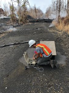
Notice that both forces come from the lithosphere, the cold “lid” of the tectonic convection system. In this way, the driving mechanism of plate tectonics differs somewhat from conventional convection (eg the pot on the stove) where there is a concentrated heat source at the base. However, there are convection systems that work in a similar way, notably certain volcanic lava lakes that have a solid crust on molten lava below. An example is Kiluea volcano in Hawai’i. There, time-lapse camera systems have recorded spreading centres, subduction zones, and transform faults forming and reforming on the lava survface. The analogy is a good one, but not perfect, because below the solid upper layer these lava lakes are truly liquid, whereas the Earth’s mantle is a plastic solid.
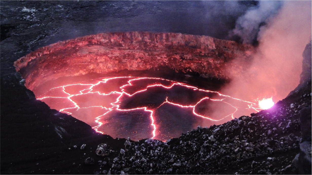
Plate movements in the past[4]
- Data from https://en.wikipedia.org/wiki/Modified_Mercalli_intensity_scale#Correlation_with_physical_quantities and Blue Planet by Skinner & Murck ↵
- Clague, J. J., Bobrowsky, P. T., & Hutchinson, I. (2000). A review of geological records of large tsunamis at Vancouver Island, British Columbia, and implications for hazard. Quaternary Science Reviews, 19(9), 849–863. https://doi.org/10.1016/S0277-3791(99)00101-8 ↵
- Arima, E. Y., St. Claire, D., Clamhouse, L., & Edgar, J. (1991). Between Ports Alberni and Renfrew: Notes on West Coast peoples. University of Ottawa Press. ↵
-
A future section may deal with controversies about tectonics in the early Earth
- Mesozoic and Cenozoic: an excellent record
- Paleozoic and Proterozoic: a fragmentary record of plate movement
- Archean and Hadean: style of tectonics is controversial
A theory that explains features of the Earth by slow movement of the continents over geologic time. The theory of continental drift has largely been incorporated into the later theory of plate tectonics, which also explains movements of the ocean floor.
A theory that the Earth has a lithosphere that is divided into relatively rigid moving plates that interact along plate boundaries
A new collection of objectives, methods, and theories for a scientific discipline, developed during a scientific revolution
Global positioning system (GPS): A satellite-based navigation system that has additionally provided evidence of plate motion
The variation in elevation from place to place on the surface of the Geosphere, on land. (The corresponding measurement of the seafloor is bathymetry.)
Measurement of the depth of the sea floor.
A graph representation of the prevalence of different elevations across Earth’s surface.
Of silicate minerals and rocks, having large amounts of magnesium and iron; mafic rocks have silica contents of 45–50%.
An igneous rock or magma with between 52% and 65% silica
Igneous rock or magma with more than about 65% silica. Felsic rocks typically contain quartz
with potassium and/or sodium feldspar.
A mountain belt formed by shortening of the crust.
The fringe of a continent were it shares a boundary with oceanic crust.
An area of shallow sea (<200 m) at the edge of a continent, underlain by continental crust.
Deep troughs on the ocean floor where oceanic lithosphere is subducted at a convergent plate boundary
A chain of volcanic islands formed above a subduction zone.
Elevated regions on the ocean floor centred on divergent plate boundaries.
The study of the Earth using physical properties to probe parts that cannot be directly observed.
The rigid outer part of the Geosphere that is divided into plates, consisting of the crust and outer layer of the mantle
A rigid, moving part of the Lithosphere
A localized region at the Earth's surface located above an unusually hot part of the mantle.
global positioning system
A fundamental force between all masses in the universe
A device used to measure the slight variations in gravity seen at Earth’s surface due to differing rock density below.
Variations in the force of gravity due to differing rock densities below.
A vertically hanging thread suspending a weight, used to define the vertical direction using the force of gravity.
The layer of the mantle lying beneath the lithosphere and capable of plastic flow
The behaviour of upper layers of the Earth as if floating on the more deformable Asthenosphere below; lower density material corresponds to higher elevations.
The phenomenon in which the lithosphere rises when a surface load (such as an ice sheet) is removed.
Elevated terraces along shores that arise uplift, typically due isostatic rebound following the removal of glacial ice.
A measure of the resistance of a fluid to shearing; measured as the force concentration needed to achieve a given velocity gradient. In everyday terms, a measure of hhow 'thick' a fluid is.
A region within which the direction of magnetic force can be determined
The magnetic field produced by a magnetized body with north and south poles on opposite sides
The study of preserved magnetism in ancient rocks
The direction relative to the north of Earth’s magnetic field.
The steepness of Earth’s magnetic field.
The north and south poles of Earth's magnetic field
Permanent magnetism that was acquired at the time of rock formation and preserved until the present day.
An iron oxide mineral with the formula Fe₃O₄
The extrusive product of mafic magma. Basalt has a fine grain-size and a dark colour.
The temperature at which a mineral acquires the ambient magnetic field orientation during its cooling; for the common magnetic mineral magnetite the Curie point is 570oC.
Daughter isotope
An isotope produced as a result of isotopic decay.
The path of one of the Earth’s magnetic poles over geologic time, as it appears relative to a
given continent
Geologically rapid exchange of the polarity of Earth’s magnetic north and south poles.
Regions where Earth’s magnetic field is stronger or weaker than predicted by a simple dipole model of the magnetic field.
The hypothesis that symmetrical patterns of linear magnetic anomalies on the ocean-floor have been produced by ocean-floor spreading combined with reversals of the Earth's magnetic field.
A fracture in Earth’s crust where bodies of rock may slide past each other.
The chance that an earthquake of a given magnitude will occur in a given area during a given time interval.
A change in shape or volume
Stress that acts with different intensity in different directions
Deformation where strain and stress are proportional. Energy is then stored in elastically deformed rocks and released when the stress is reduced.
The relative movement of blocks on either side of a fault
An event in which stored elastic energy is rapidly released by sudden movement on a fault
surface
A slipped region of a fault surface
Disturbances generated by a natural earthquake or by artificial means, that propagate as vibrations through the Geosphere and over its surface.
The point within the Earth where an earthquake begins, and from which seismic waves radiate
The focus of an earthquake; the point within the Earth from which seismic waves begin to radiate.
A point on the Earth's surface located vertically above the focus, or hypocentre, of an earthquake
A device used to create a record of shaking resulting from an earthquake
A device used to measure shaking resulting from an earthquake
Earthquake intensity measures the amount of ground shaking at a point. Intensity typically decreases away from the focus of the earthquake.
A scale for measuring the intensity of an earthquake
The increase in the rate of movement of an object
A value which is independent of the amount of material under consideration, such as temperature or chemical concentration.
A measure of the energy release from an earthquake, scaled to the logarithm of displacement at a standardized distance.
A measure of earthquake magnitude based on displacement at a standardized distance; in modern work, largely superseded by moment magnitude
A scale of earthquake size that depends on the amount of slip and the slipped area of the fault surface. The moment magnitude is commonly calibrated to the older Richter scale but gives a more precise measure of earthquake size.
Seismic body waves in which the vibration direction is parallel to the propagation (travel) direction.
Seismic body waves in which the vibration direction is at 90° to the propagation (travel) direction
The layer within the Earth or other inner planet that overlies the core and makes up the majority of the planet, composed chiefly of magnesium- and iron-rich silicates
The layer of the core directly below the mantle, composed mainly of liquid iron.
Seismic waves that travel along the surface of the Geosphere
Seismic surface waves that produce vertical motions of the ground surface.
Seismic surface waves in which motion is horizontal and perpendicular to the wave propagation direction
A wave on the ocean surface resulting from an earthquake, volcanic eruption or a landslide.
A thin, surface layer of the Earth that lies above the Moho; differentiated into thicker, lighter continental crust and thinner, denser oceanic crust
The central part of the Earth below about 2900 km from the surface, composed largely of metallic iron
The portion of the Lithosphere below the Moho and above the Lithosphere-Asthenosphere boundary
The portion of the mantle below ~650 km, below the transition zone.
The behaviour of seismic waves that encounter a boundary within the Earth, causing some of the energy to return away from the boundary on the same side as their source
The resistance of a substance to seismic waves passing through it; acoustic impedance is a
function of the substance’s density multiplied by the velocity of seismic waves travelling through
the material.
A major discontinuity and seismic reflector ~2900 km below the Earth's surface, separating the silicate mantle from the metallic core
A phenomenon affecting all kinds of waves, whereby waves impinging obliquely on a boundary where their velocity changes experience a change in the direction of wave propagation
Moho: The boundary at the base of the Earth’s crust where seismic P-waves abruptly increase in velocity..
Mohorovičić Discontinuity: The boundary at the base of the Earth’s crust where seismic P-waves abruptly increase in velocity.
Utramafic rock composed mostly of pyroxene, usually together with olivine
Magma or igneous rock with a silica content of less than 45%
A silicate of iron and/or magnesium with separate silicate tetrahedra in its structure; (Mg,Fe)₂SiO₄.
A zone in the upper mantle where both P- and S-waves slow down, corresponding approximately to the Asthenosphere
An area on the Earth's surface where seismic body waves from an earthquake are blocked by the Core
The fourth planet from the the Sun
The boundary between two plates moving apart from one another; divergent boundaries are commonly the sites of rift valleys and ocean-floor spreading.
Melting of rock material to produce a mixture of solid and liquid.
Thinner crust is composed mostly of mafic rock.
A plate boundary where relative plate motion is parallel to the boundary.
A fault where the side opposite to an observer appears to be moving to the observer's right.
Dextral: fault motion such that the far wall of a fault appears displaced to the observer's right
Fault motion such that the far wall of a fault appears displaced to the observer's left
Sinistral: fault motion such that the far wall of a fault appears displaced to the observer's left
The plate tectonic process whereby one plate descends beneath another as plates converge
A deep, linear feature of the ocean floor that marks a convergent plate boundary
The behaviour of upper layers of the Earth as if floating on the more deformable Asthenosphere below; lower density material corresponds to higher elevations.
A convergent plate boundary where one plate descends beneath another.
The boundary between two plates moving towards one another. Convergent boundaries are the sites of subduction of one plate beneath the other.
A chain of volcanoes that lies above a downgoing slab of lithosphere at a subduction zone
A sloping zone of deep earthquakes associated with a convergent plate boundary
An uprise of mantle material that cause a hotspot in the Earth’s lithosphere.
A group of hard silicate minerals with isolated silicate tetrahedra containing combinations of aluminum, iron, magnesium, calcium and other elements. Garnets are most common in metamorphic rocks
A group of mainly ferromagnesian single-chain silicate minerals common in mafic rocks
A metamorphic rock formed at high pressure and moderate to high temperature; components of feldspar become dissolved in red garnet and green pyroxene
A cycle in which the products of a process act as inputs increasing the activity of the same process
