
21 Time and the Geosphere
This chapter is a near-final draft.
Learning Outcomes
By the end of this section you should be able to:
- Determine the relative timing of events from features in the Geosphere;
- Explain the principal methods for absolute (numerical) dating of rocks, and their limitations;
- Calculate simple age determinations using half-life or decay constant.
Geologic time
Earth science deals in very long periods of time, termed geologic time, or geological time. Ideas of geologic time were developed in the 1800s, but geologic time scale had no numbers when it was developed; it was a relative time scale that indicated what was older and what was younger, but had no units. The discovery of radioactivity gave Earth scientists the ability to measure geologic time, beginning early in the twentieth century. However, not all Earth materials are capable of being dated using radioactive isotopes, so relative methods of dating events are still important.
In the following account, we follow this history, beginning with concepts of relative time, and continuing with an examination of isotopic or absolute dating methods.
The lengths of time revealed by isotopic dating are extremely long: billions of years. Human understanding of time has evolved to deal with events that occur in seconds, ranging up to periods in years and decades. This makes it difficult for our brains to comprehend the enormous lengths of time revealed by the Geosphere. These lengths of time, far beyond human experience, are sometimes referred to as deep time, a term coined by scientific writer John McPhee in his book “Basin and Range”, published in 1981.
To handle these great lengths of time, Earth scientists use some special units and abbreviations.
- Times measured as thousands of years before the present day are specified using the unit kilo-annum, abbreviated to ka.
- Times measured as millions of years before the present day are specified using mega-annum, abbreviated to Ma.
- Times measured as billions of years before the present day are specified using giga-annum, abbreviated to Ga.
Notice that all these units imply times measured backwards from the present day. Therefore, it’s technically incorrect to say “66 Ma ago”, because “Ma” includes the sense of “ago”. For time durations that don’t end at the present day, it’s more correct to use “yr”, as in “The Paleozoic Era lasted for about 290 Myr.”
Relative timing of events
Some of the earliest conclusions about geologic time, long before the advent of isotopic dating, were drawn from observations of layered rocks. Pioneers of geology, working in the 18th century, developed some basic principles for the interpretation of layered rocks.
Order of strata
Sedimentary rocks mostly contain layers that record environmental change over time. A layer is also called a stratum; multiple layers are strata.
In many parts of the world, a hierarchy of strata can be recognized.
- Layers less that 1 cm thick are laminae (singular lamina).
- Thicker layers at the scale of rock outcrops are beds.
- Layers at the scale of maps are called formations and groups.
The principle of original horizontality states that sedimentary strata were initially deposited on the approximately horizontal surface of the geosphere. If we find strata that are tilted we can deduce that a tilting event, or events, occurred after the deposition of the strata.
The principle of superposition states that the lowest sedimentary strata in any succession of strata were the first to be deposited, and the higher strata are younger.
Correlation by lithology
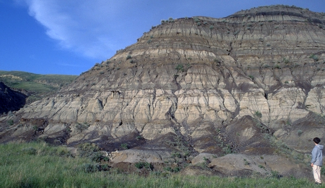
The succession of sedimentary layers in an area is efficiently illustrated in a stratigraphic column. An examples is shown in the figure.
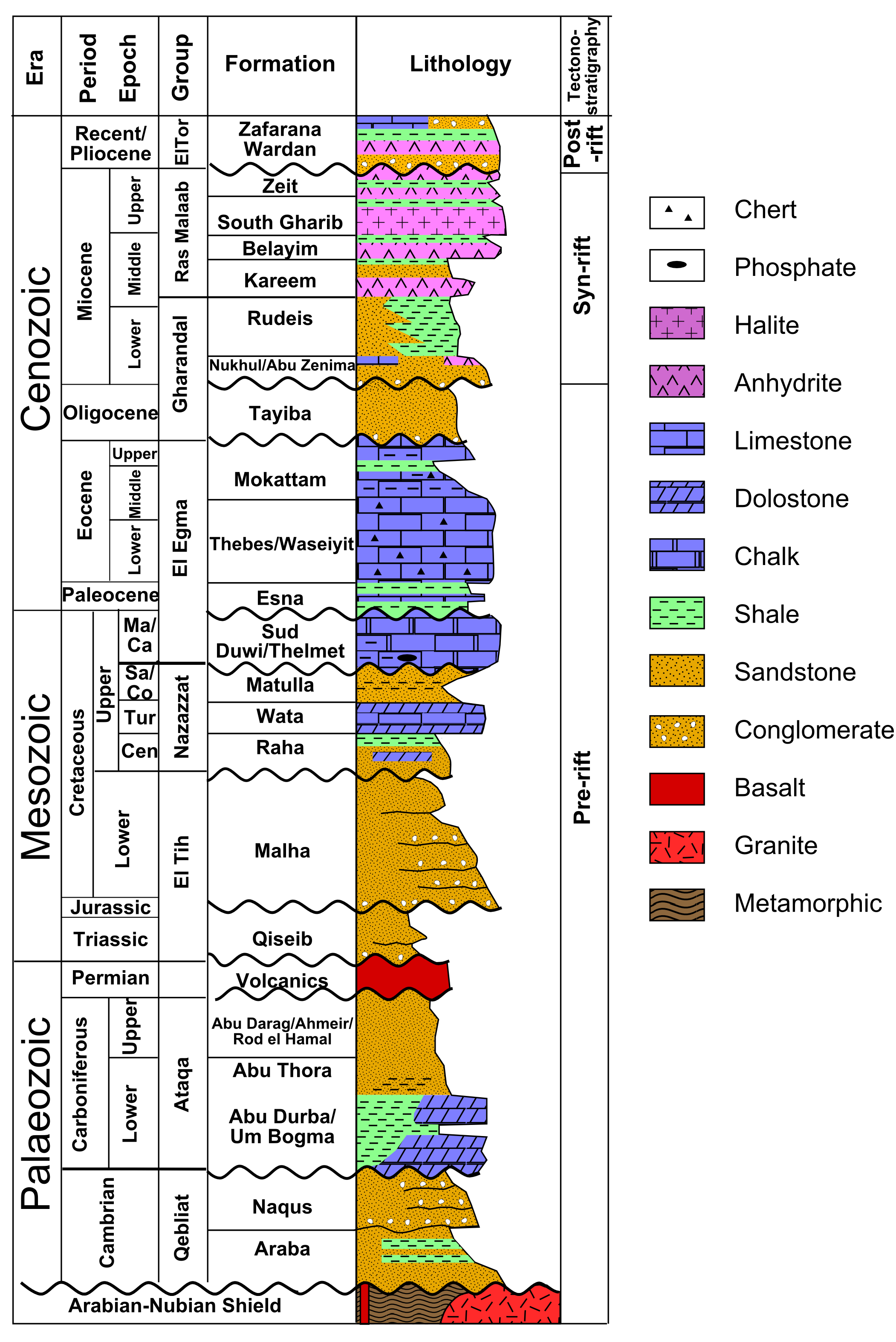
Often, it is difficult to trace strata over long distances, because they may be obscured by vegetation, covered by other rock units, or removed by later erosion. Under these circumstances, it is helpful to compare stratigraphic columns in order to correlate strata. Correlation is the process of comparing successions of layers in different places.
If the succession of layers is very similar in two places, as in the example shown in the figure, a geologist may conclude that the layers were originally continuous from one to the other.
Correlation by fossils
Long before the discovery of evolution by natural selection, it was realized that strata can be correlated by means of the fossils they contain. Most of the periods in the younger part of the geologic time scale (the Phanerozoic Eon) were identified based on distinctive fossils, and correlation by fossils continues to be an important part of figuring out the history of sedimentary rock deposition.
The best fossil groups for correlation purposes have certain characteristics in common.
- They must be abundant, with hard parts that are readily preserved, so that they can easily be found.
- They need to have wide geographic distribution, so that correlation can be achieved between distant parts of the world.
- They should show no strong biogeographic provinciality.
- They should be marine, as most sedimentary rocks are deposited in the sea.
- They should be free swimming or planktonic (floating in the pelagic zone of the ocean).
- They should undergo rapid evolutionary change leading to the development of recognizable species.
An example of a group that excels in these respects is an order of molluscs called ammonites, that lived in the Mesozoic Era. The ammonites were marine organisms related to the modern pearly nautilus, and more distantly related to squid and cuttlefish. They thrived in the Mesozoic seas but became extinct at the same time as the dinosaurs at the end of the Mesozoic Era. During the time of their existence, they evolved rapidly, producing new species every few hundred thousand years or so, allowing the strata to be divided into many biostratigraphic zones. Although the ammonites were somewhat provincial, with different species living in tropical and temperate oceans, many species ranged over most of the Earth, allowing them to be used for global correlation.

Cross-cutting relationships
Additional constraints on the order of events in the history of our planet are provided by what are known as cross-cutting relationships, typically places where strata have been cut off or modified by events that occurred after deposition.
Unconformities
An unconformity is an ancient erosion surface, typically formed where older rocks were exposed to erosion at the Earth’s surface and then covered by younger strata. An unconformity represents a gap in the stratigraphic record. It therefore gives evidence for three different events in the history of a region:
- Formation of rocks below the unconformity surface. Note that these may be igneous, sedimentary, or metamorphic;
- Erosion, sometimes accompanied by tilting or other movements of the Geosphere
- Deposition of younger rocks above the unconformity, usually sedimentary.
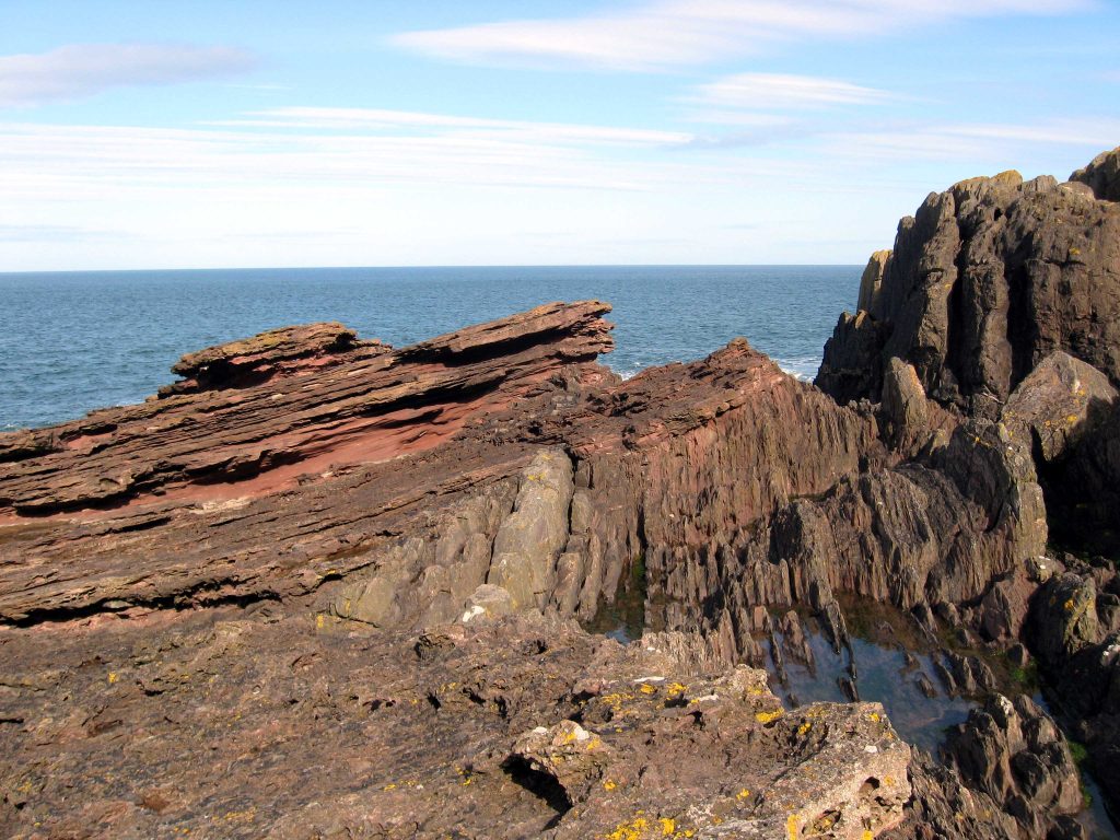
James Hutton, the 18th century developer of the principle of uniformitarianism, identified several unconformities in his native Scotland. The most famous, at Siccar Point, shows grey marine clastic sedimentary rocks, that were tilted almost to vertical, eroded, and then overlain by younger red layers that were probably deposited by river systems that flowed across the land surface. These younger strata contain clasts eroded from the older strata below the unconformity surface. Even the younger strata are not horizontal. This shows that the entire package of rock was tilted again, at some time between the depostion of those strata and the present day. At the present day, waves pound the beach during storms so erosion is occurring once again.
Igneous intrusive relationships
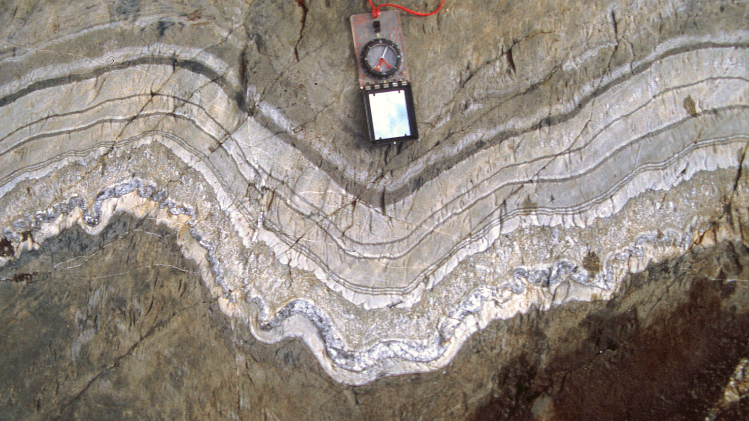
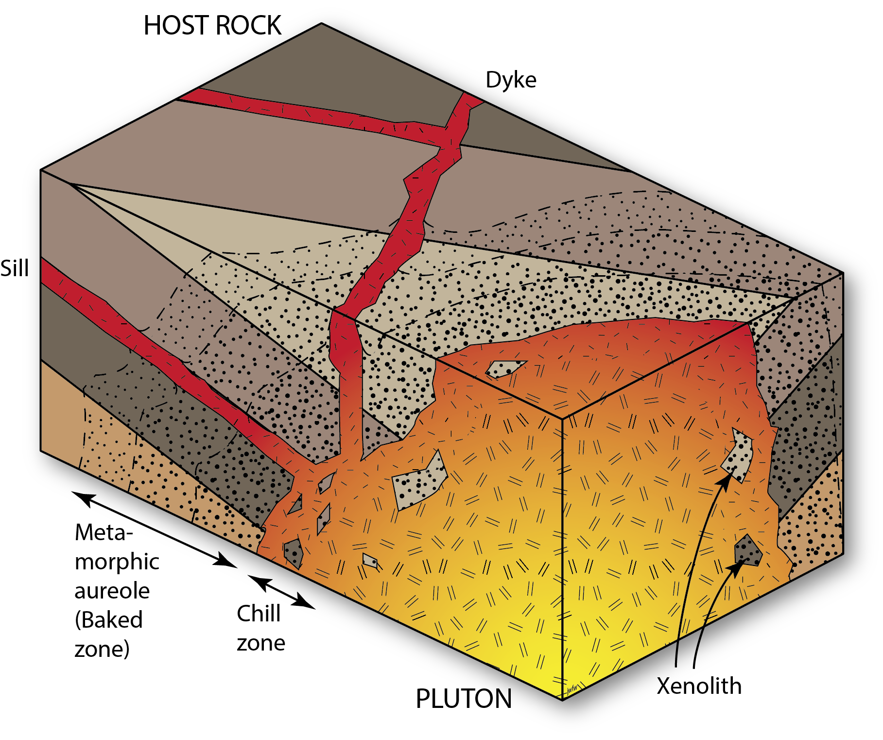
Igneous intrusions also form cross-cutting relationships. Plutons may cut off the layers in surrounding sedimentary rocks, and cause contact metamorphism, showing that the sedimentary rocks were there first, and the intrusion was second. Smaller cross-cutting intrusions – dykes – record similar relationships.
Note that igneous intrusive contacts are not unconformities. Although there is certainly a discontinuity in the geosphere at the edge of an intrusion, we reserve the word unconformity for discontinuities produced by erosion that was followed by deposition of strata on the erosion surface.
Faults
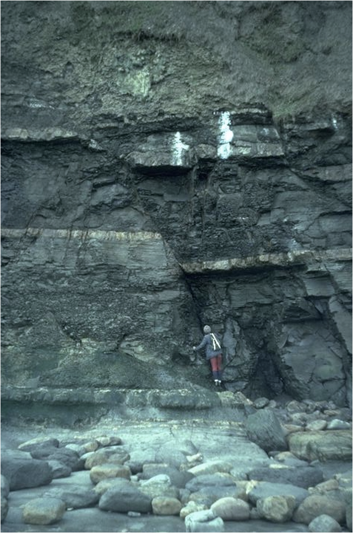
Faults are brittle fractures that form in the outer parts of the Geosphere due to tectonic movements[1]. They are cracks where there has been relative movement of rocks on either side, in any direction that is parallel to the fracture surface. When faults cross-cut strata they show that the faulting process must have occurred after deposition of the strata, providing another piece of evidence that can be used in reconstructing the history of a region.
Geologic time scale[2]
The most recent part of Earth history, the Phanerozoic Eon, was subdivided into eras and periods as a result of investigations into fossils, together with the principle of superposition and the use of crosscutting relationships, during the 1800s. Much of this work was done before Darwin’s proposal of a mechanism for evolution, and all of the periods were defined before the discovery of radioactivity. Therefore, the numerical ages of the divisions in the time scale were not originally known, but their sequence in time was well defined.
Early Earth scientists tended to assume that the divisions of the time scale were either products of divine creation or were separated by worldwide catastrophes, and therefore that major changes in environments would occur globally at the same time. We now know that this is incorrect; although some boundaries (such as the Mesozoic–Cenozoic boundary at ~66 Ma) are marked by global catastrophes, others are not. Arguments about the placement of boundaries have resulted in revisions to the time scale since the nineteenth century. A most current version can be found at www.stratigraphy.org/chart
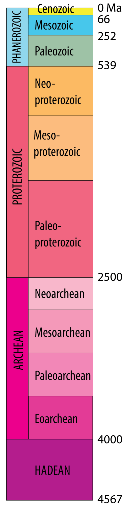
Subdividing earlier parts of Earth history (“Precambrian time”) has proved more difficult, because of the scarcity of metazoan fossils. In some parts of the world early subdivisions were based on the presence of unconformities, but in modern time scales Precambrian time is divided into two or three Eons based on isotopic ages: Proterozoic, Archean and (in most systems) Hadean.
Numerical dating using isotopes
Prior to the discovery of radioactivity, the geologic time scale was entirely relative: it showed what was older and what was younger but no numerical ages were applied. There was a great deal of argument about the age of the Earth, which was generally assumed to have internal heat (geothermal energy) only as a result of steady cooling since the origin of the solar system.
The discovery of radioactivity provided both a means of measuring the absolute or numerical age of certain rocks, but also an explanation for the origin of a large proportion of geothermal energy, which requires a heat source that continued after the origin of the solar system. Radioactive elements within the Earth provide that heat source.
Isotopic methods: Atomic structure
To understand radioactivity we must understand some aspects of the structure of individual atoms.
All matter is composed of about 90 naturally occurring elements. Atoms are the smallest individual particles of an element, about 10-10 m diameter. [3]
Each element has a unique atomic number, which is the number of positively charged protons in the atomic nucleus. If the atom is uncharged then this number will equal the number of electrons in the electron cloud, but this may vary as an element becomes ionized.
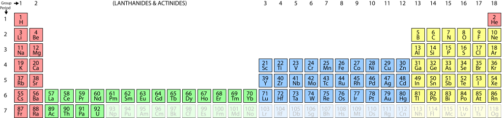
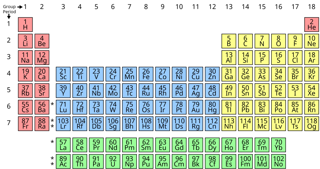
The periodic table shows all the elements in order of atomic number, from hydrogen (element 1) through to uranium (element 92) and beyond into elements that are not known naturally but which have been synthesized by humans. In the periodic table the elements are arranged so that elements with the same electron configuration in the outer electron shell occur in the same column. This groups elements with similar chemical properties together.
However in this section we are more concerned with what goes on in the nucleus. For all elements except hydrogen, the nucleus must also contain neutrons, particles without electric charge that play a role in binding the nucleus together. A neutron has about the same mass as a proton, and both are much more massive than electrons. Therefore, the number of protons plus neutrons is a measure of the mass of a nucleus and is known as the atomic mass number. For example, most atoms of carbon have 6 neutrons in addition to the 6 protons so the atomic mass number is 12. A closely related concept is atomic weight which measures the actual mass of the atom[4].
For any element the number of protons is constant, but in most elements the number of neutrons can vary. For example, carbon occurs in forms with 7 and 8 neutrons in addition to the standard 6, producing isotopes of carbon. Isotopes are usually referred to by their atomic mass number, so we speak of carbon-12 (the most abundant isotope), carbon-13, and carbon-14. Note that these can also be written as 12C, 13C and 14C.
Because all three isotopes of carbon have the same number of protons, and therefore the same number of electrons in the electron cloud that is responsible for their chemical properties, they have almost identical chemical and physical properties. However, 3C and 14C are a little heavier than 12C, so they tend to be fractionated during certain reactions, especially those that generate gases (which often capture slightly more of the light isotope). This can be useful in tracking the origin of carbon dioxide, methane, and carbonate ions in the carbon cycle.
Radioactive decay
Certain isotopes of many elements are unstable: the nucleus has a tendency to break down or decay, changing the atomic number. In the process, particles and energy, known as nuclear radiation, are emitted. The phenomenon is called radioactivity.
For a given isotope the rate of radioactive decay is predictable, because for any one atom, the chance of decay in a given time is constant. Therefore, provided a sample has a large number of atoms, the laws of probability govern what proportion of its atoms will decay per year. If we can measure the number of remaining atoms, and we have some way to estimate the number of atoms that were present when a rock formed, we can figure out the age of the rock. This process is known as radiometric or isotopic dating.
To take a common example, consider the element carbon, symbol C. The atomic number of carbon is 6 and it occurs in three common isotopes.
| Isotope | Stable or unstable | Protons | Neutrons | Abundance |
| 12C or Carbon-12 | stable | 6 protons | 6 neutrons | 99% of natural C |
| 13C or Carbon-13 | stable | 6 protons | 7 neutrons | 1% of natural C |
| 14C or Carbon-14 | Decays with a half life of 5730 years | 6 protons | 8 neutrons | 1.3 x 10⁻¹⁰ % of natural C |
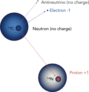
Carbon-14 is unstable. Within the nucleus, one of the extra neutrons may spontaneously change to a proton by expelling a high-energy electron, which may be detected as beta radiation. The atom therefore changes to Nitrogen-14, which is known as the daughter isotope. (Carbon-14 is the parent.)
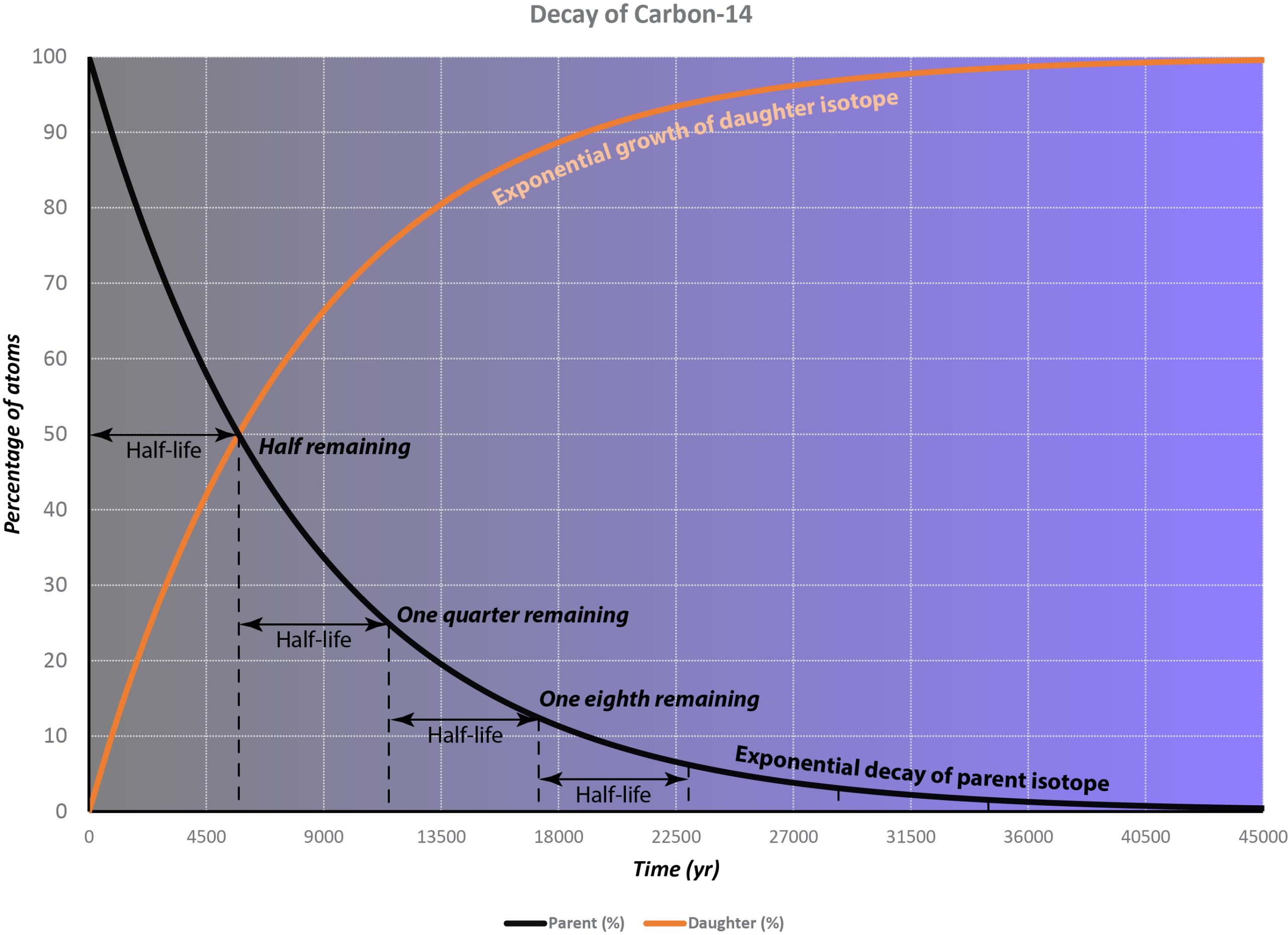
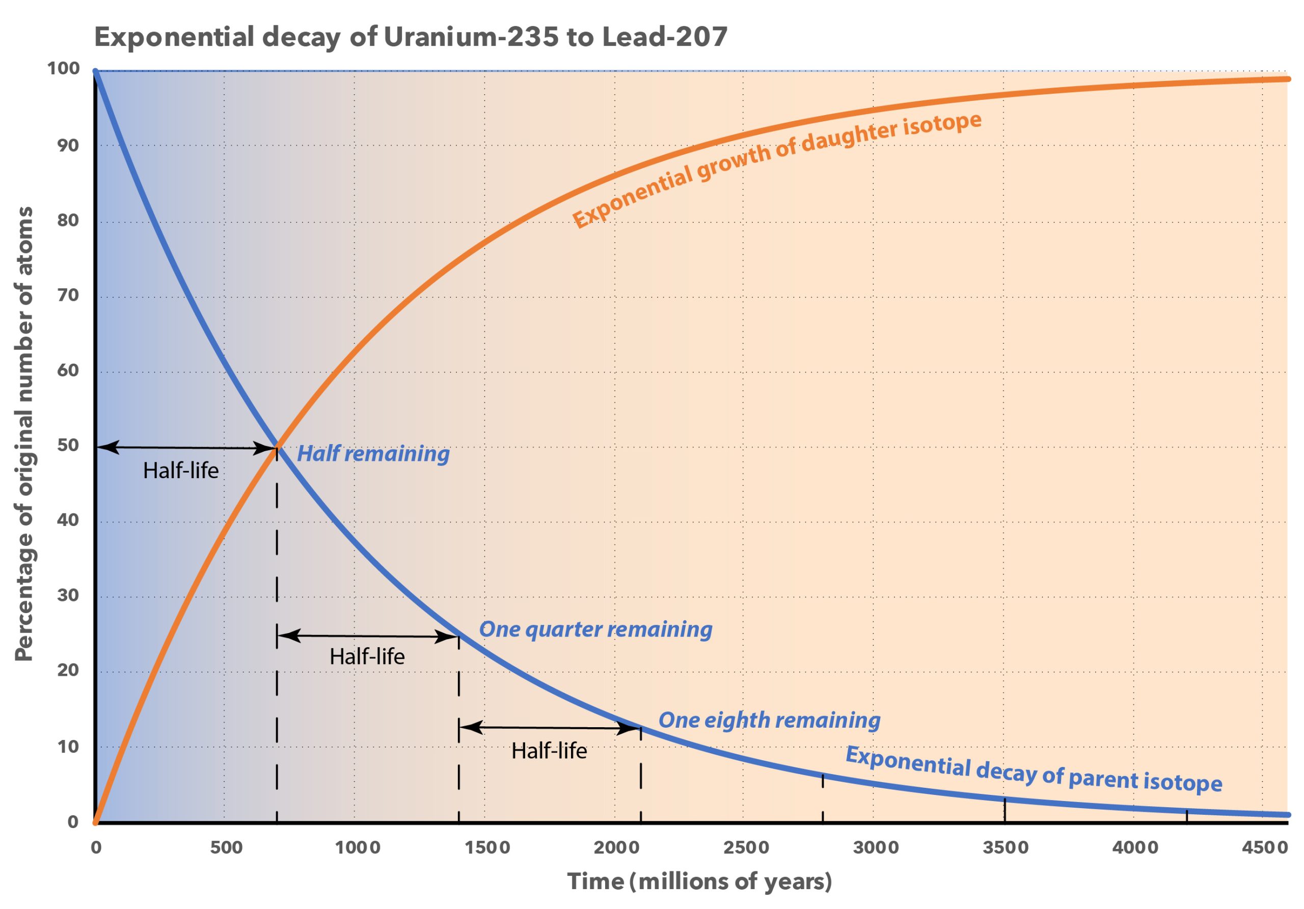
This process is completely random; any given carbon-14 atom has the same chance of decaying within a given time period. The result is that for any sample of carbon-14, half the atoms decay within 5730 years, a period known as the half-life of Carbon-14. During the next 5730 years, half of the remaining atoms will decay, leaving a quarter of the original amount. After three half-lives only one eighth of the parent will remain, and so on.
This type of decay pattern is known as exponential decay. It’s easy to calculate the amount of isotope remaining after a whole number of half-lives, by dividing by two as in the previous paragraph. For general calculations, we can use a decay constant λ and the following formula:
N = N0e-λt
where N is the number of atoms remaining after time t, N0 is the original number of atoms, and e is the mathematical constant 2.71828, the base of the natural logarithms.
To find the age, knowing the original and final amounts of the parent isotope we can use

The decay constant is related to half life (t1/2) by……
λ = ln(2) / t1/2
or λ = 0.693 / t1/2
What are the requirements for determining the age of a material using an unstable isotope? We need to know, or be able to calculate N and N0. In many cases we can measure N, but for most methods used on minerals we can’t measure N0. However, if we can measure the amount of daughter isotope produced by radioactivity (D*) we can calculate N0 by adding the amounts of remaining parent and daughter isotopes. So the quantities we need to know to come up with an age are
- The half-life or decay constant
- The remaining amount of the parent isotope
- Either
- The initial amount of the parent isotope or
- The amount of daughter isotope formed by isotopic decay
Dating methods
In this section, we will look at some examples of isotopic dating methods.
Radio-carbon dating
Radio-carbon dating relies on the fact that carbon-14 is continuously produced in the atmosphere by impacts between solar neutrons and nitrogen-14 atoms. The proportion of carbon-14 in the atmosphere stays approximately constant at 1.3 x 10⁻¹². This is a tiny amount, but it can be measured either by detecting beta-radiation from the decaying atoms or by directly counting atoms in a mass spectrometer.
- The half life of carbon-14 is 5370 years so the decay constant λ is 3.8394 × 10⁻¹² per second.
Carbon is continuously captured from the atmosphere by plants, so wood captures the same proportion of carbon-14 as the atmosphere. Organisms that build skeletons of calcium carbonate also capture carbon that was recently in the atmosphere. Therefore, both organic carbon and oxidized, carbonate carbon can be dated.
However, the half-life of carbon-14 is short in comparison to the age of the Earth, so radio-carbon dating cannot practically be used to date materials older than about 50,000 years. Another limitation is that the proportion of carbon-14 in the atmosphere has fluctuated slightly over time because of major solar flares. These fluctuations can be taken into account using dates obtained by counting tree-rings (dendrochronology) or varves deposited in glacial lakes to calibrate radio-carbon ages.
Uranium-lead zircon dating
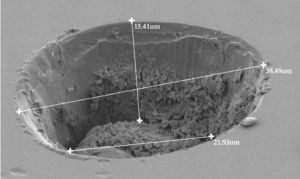
Uranium-Lead dating is often carried out using the zirconium silicate mineral zircon ZrSiO4.
Zircon crystals typically form when felsic magma solidifies. Zirconium ions have same charge and almost the same size as uranium (U) ions, so if any uranium is present in the magma it is usually captured by zircon. However, the decay product of uranium is the element lead (Pb) and lead is not easily accommodated in the zircon crystal lattice. (Furthermore, if some lead is incorporated when a zircon crystal grows, it’s possible to detect this and estimate how much by measuring an isotope of lead that is not a product of radioactive decay).
![]()
![]()
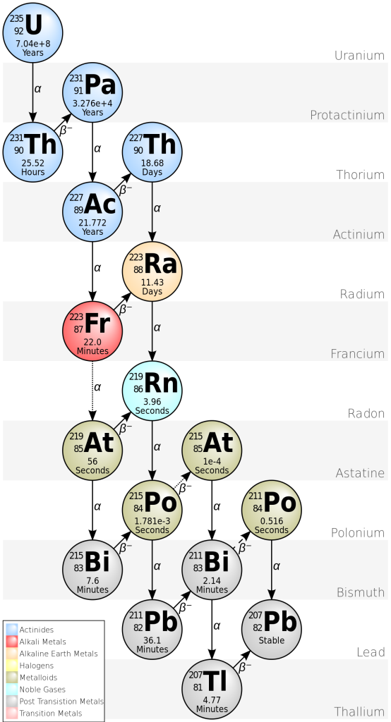
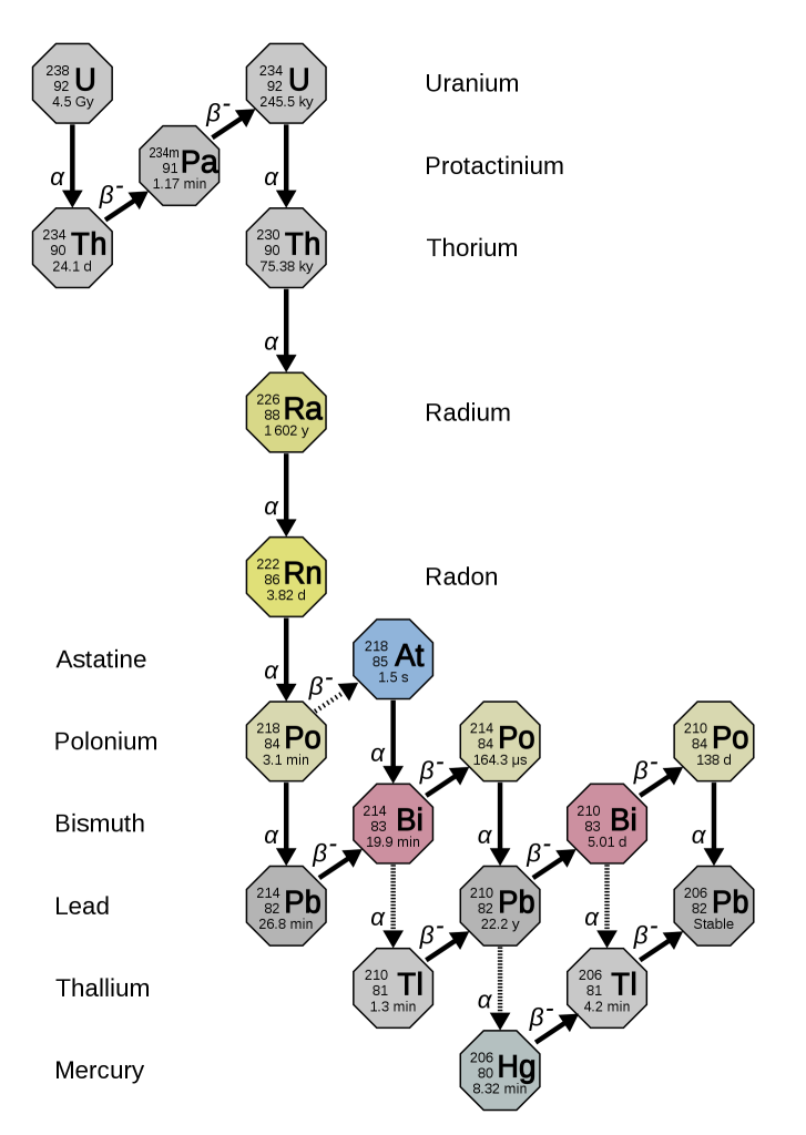
There are two decay processes that produce lead from uranium. For both isotopes, there is a long chain of intermediate nuclear reactions, but it’s possible to combine all these reactions to make a single half-life (and decay constant) for each series.
235U decays to 207Pb (t1/2 = 704 million years).
238U decays to 206Pb (t1/2 = 4468 million years)
This means that each crystal of zircon actually contains two isotopic “clocks”, which provide an independent check on the results. If lead has been lost at any stage, the two decay processes give different results.
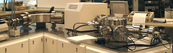
To measure the amounts of the various isotopes, zircon crystals may be dissolved and evaporated, or they may be ablated using a laser. The released atoms are counted using a mass spectrometer, which is able to separate atoms according to their atomic weights.
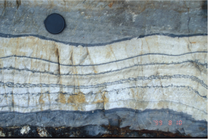
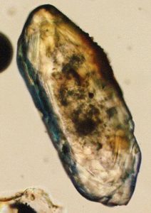
For example, the figure shows a layer of tuff (solidified volcanic ash) from the Northwest Territories in Canada. (The same outcrop is shown as an example of correlation in the section on relative dating.) Zircon grains were separated from the rock and analysed with a mass spectrometer for their uranium and lead isotopes, to determine the amounts of parent and daughter isotopes. The resulting ages from the two isotopic systems agree within a few million years, giving an age of 2661 ± 2 Ma, in the late Archean. Because the tuff is so easily correlated, the same age can be interpreted for the other outcrops as well.
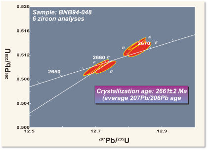
Notice that isotopic ages are always subject to a statistical error. Both the decay process and the analysis involve random events affecting large numbers of atoms, so repeated measurements give very slightly different results. The errors are typically quoted as 95% confidence limits – the range within which, if the measurement were repeated multiple times, the answer would lie 19 times out of 20.
Useful isotopic systems
The following table summarizes the most-used methods of isotopic dating in Earth science.
| Parent | Daughter | Half-life (million years) | Materials | Uses |
| Uranium-238 | Lead-206 | 4468 | Zircon | Igneous rocks |
| Uranium-235 | Lead-207 | 704 | ||
| Rubidium-87 | Strontium-87 | 47000 | Mica, Feldspar | Igneous rocks |
| Potassium-40 | Argon-40 | 1251 | Mica Amphibole | Igneous, metamorphic rocks |
| Carbon-14 | Nitrogen-14 | 0.00573 | Organic matter, calcium carbonate | Young fossils, wood, historical artifacts |
| Rhenium-187 | Osmium-187 | 41600 | Sulfides, organic matter | Mineral deposits, hydrocarbons |
| Lutetium-176 | Hafnium-176 | 37100 | Igneous rocks, Zircon | Crustal evolution |
| Samarium-147 | Neodymium-143 | 68.7 | Rocks generally | Crustal evolution |
It’s important to note that not all rocks can be dated. To use isotopic dating to date a rock…
- Mineral grains must have formed at the same time as the rock;
- The required isotopes must be present in measurable amounts;
- Neither parent nor daughter isotopes may have leaked out of the rock after its formation.
Because most clastic sedimentary rocks contain minerals derived, by erosion, from older parts of the Earth, it’s typically not possible to date them by isotopic means. An exception is the Rhenium–Osmium method, which is in some cases able to date organic matter buried with sediment. However, fossil time-scales are now quite well calibrated at places where fossils and volcanic rocks occur together, so for Phanerozoic rocks without radiogenic minerals, relative and absolute dating methods can often be combined to deduce an age..
Other methods for numerical ages
There are several methods for measuring geologic time that involve counting phenomena that repeat regularly in time: usually the weather cycles of summer and winter, but otherwise involving events as short as a month (for example when cycles of neap and spring tides can be identified in sedimentary layers) or as long as tens of thousands of years (for example, Milankovitch cycles of climate change). These are methods of absolute dating because they give a numerical answer in years, although they are often achieved using observations of sedimentary rocks and fossils that are more commonly used for relative dating.
Many of these methods can only be applied under rather special circumstances, when environments remain the same through many cycles. We will review only the most important.
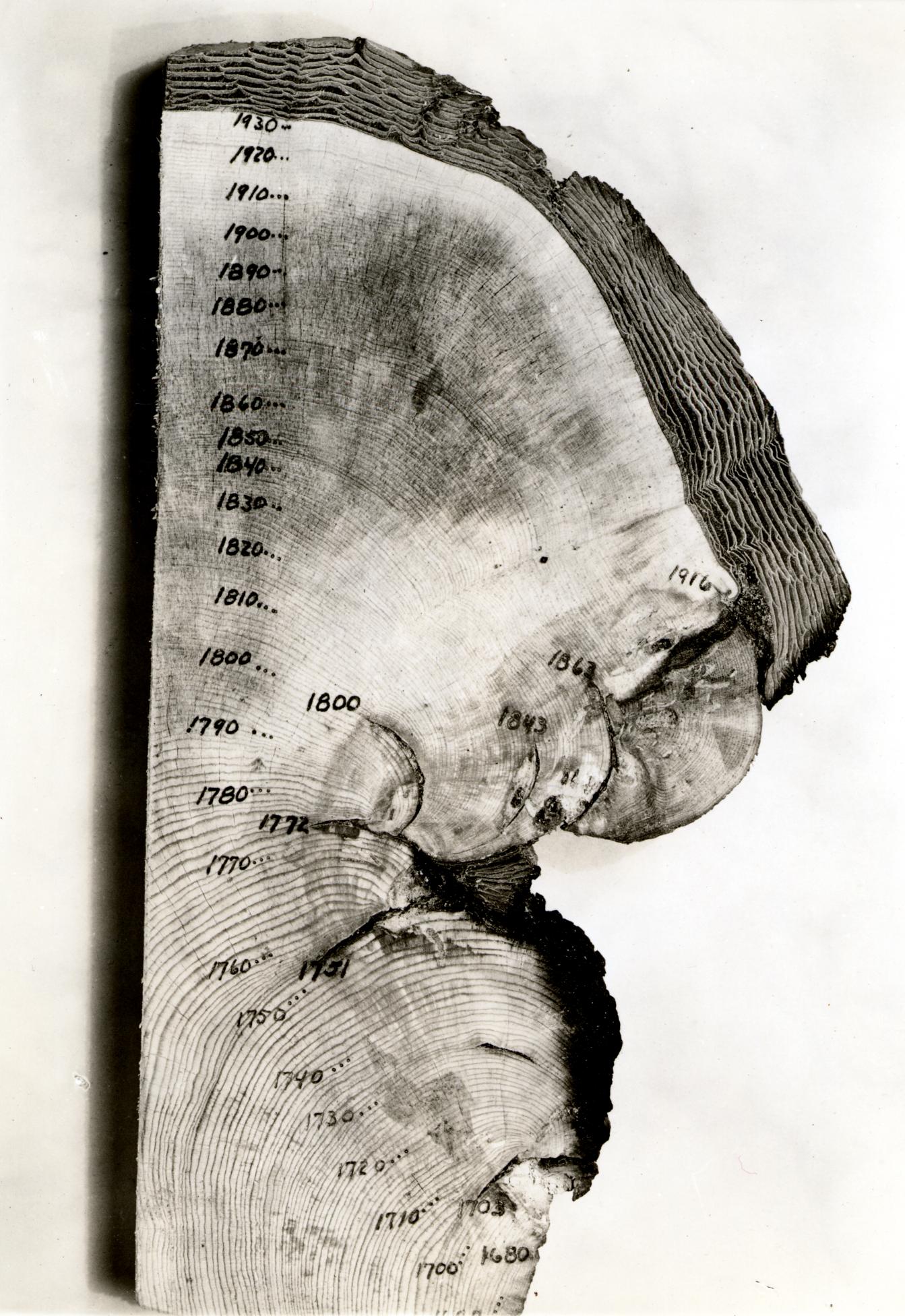
Annual growth rings in organisms
Many organisms show changes in their growth that coincide with the seasons. The most well known are the layers in the stems of woody plants, commonly known as tree rings. Fluctuations in climate produce changes in the characteristics of tree rings, and these patterns can be correlated from tree to tree, and with historical wood samples. By correlating overlapping wood samples it has been possible to build a pattern of tree rings that goes back 10,000 years in some areas. This technique, known as dendrochronology has been used both to directly date historical samples of wood, and to calibrate the radio-carbon time scale, which is subject to error as the proportion of 14C in the atmosphere has fluctuated slightly over time.
Corals are another group that shows annual growth layers. These have been used to determine how long ancient corals grew, and also, in recent samples, to calibrate the radio-carbon scale.
Layers in ice and glacial sediments
Some glaciers contain annual layers marked by winter accumulation of snow and intervening summer seasons when the ice formed a hard surface, or even melted slightly. These layers may be preserved within a glacier, and can be counted, starting with the most recent year, in ice cores. Sometimes volcanic ash layers from known eruptions can be used to check the record. Enclosed gas bubbles may be used for many purposes, including measuring atmospheric composition over time and (as in the case of dendrochronology) calibrating radio-carbon ages.
Periglacial lakes also contain annual layers, because glacier ablation is faster in the summer, typically producing a flood of slightly coarser sediment into each lake. The amount of organic matter preserved may also vary with the seasons. Such layers are called varves. By counting varves in Scandinavian lakes it has been possible to determine precise ages as old as 52,800 years, approximately the same range as radio-carbon dating.
- Note that not all faults are plate boundaries. Most faults form as a result of deformation near the edges of plates, but only the largest faults, that pass right through the Lithosphere, qualify as plate boundaries. ↵
- Time scale is sometimes written as one word: timescale. ↵
- Sometimes 10-10 m is referred to as an Angstrom. In the S.I. system this is equivalent to 0.1 nm (nanometres). ↵
- The actual atomic weight differs from the atomic mass number because electrons are included and because a small amount of matter is converted to energy in the construction of an atomic nucleus, but these masses are small so the two are close. ↵
Thousands of years before present; ka.
Kilo-annum; thousand years before present.
Million years before present; Ma.
Mega-annum; Million years before the present.
A billion years before present. Symbol: Ga
Billion years before the present.
Stratum (plural strata): a layer of rock, typically sedimentary
Lamina (plural laminae): a thin layer (less than 1 cm thick)
A layer of sedimentary rock more than 1 cm thick
A layer of rock that appears on a geologic map
In geologic mapping, several formations that occur together
A description of sedimentary layers in the form of a columnar diagram, with the oldest layers at the bottom and the youngest at the top
The match the sedimentary layers displayed by two or more different stratigraphic columns.
A phylum of invertebrates which typically produce shells composed of calcium carbonate; Mollusca include snails, clams, and octopus (a group that has secondarily lost the shell)
A group of cephalopod molluscs with chambered shells, similar to modern nautiloids
A subdivision of strata recognized on the basis of characteristic fossil forms.
An ancient erosion surface where younger sediment was deposited on eroded older rock
The principle that processes that operated in the Earth's past can all be explained by processes that continue to operate at the present day. Strict application of uniformitarianism in Earth science has largely been replaced by actualism
A solid fragment of sediment
A process whereby magma solidifies within the Geosphere.
Large igneous intrusions
Dyke (USA — dike): A sheet-like igneous intrusion that is not concordant with any layering in its host rock
The removal of material from a site of weathering on the Earth's surface.
A fracture in Earth’s crust where bodies of rock may slide past each other.
The current eon, following the Proterozoic, from about 539 Ma to the present day, characterized by abundant remains of muticellular organisms
Changes in the characteristics of organisms, and the Biosphere as a whole, over periods of many generations.
The tendency of unstable isotopes to decay and release radioactive particles and gamma rays.
Multicellular animals
The largest subdivision of geologic time
The number of protons in the nucleus of an atom of an element, equal to the number of electrons if the atom is not ionized
A particle found in the nucleus of all atoms: protons carry a positive charge.
The heavy, positively-charged central body in an atom of an atom.
Of atoms or groups of atoms: Having lost or gained electrons producing a positive or negative charge.
A visual representation of the known elements, by order of their atomic number. Columns represent elements having similar outer-shell electron configurations, and hence similar chemical properties
A neutrally-charged particle within an atom’s nucleus
The total number of particles (neutrons plus protons) in the nucleus of an atom
Atomic weight (relative atomic mass): The mass of an atom expressed on relative a scale in which the most common isotope of Carbon is given a value 12.
Isotopes of an element are atoms that have the same atomic number but different atomic mass, because of different numbers of neutrons in the nucleus
Having a disproportionate concentration of an isotope due to that isotope's heavier or lighter weight
The breakdown of an atomic nucleus of an unstable isotope.
Particles or electromagnetic waves released by the decay of atomic nuclei in unstable isotopes.
Radiometric or isotopic dating: determination of the age of a substance using amounts of elements involved in radioactive decay
The use of unstable isotopes with known half-lives to calculate the approximate age of a sample.
High-speed electrons released during the conversion of a neutron to a proton in an unstable
isotope
An isotope that is a product of a nuclear decay reaction
An unstable isotope which decays and yields a daughter isotope.
The amount of time required for a mass of a particular isotope to decay until only 50% of the parent isotope remains.
A reduction in the amount of material at a rate proportional to the amount of remaining material.
A constant that relates the number of atoms that undergo radioactive decay per unit time to the
total number of remaining atoms; typically represented by Greek lambda (λ)
An unstable isotope of carbon with eight neutrons. Carbon-14 is used for radiocarbon dating.
Dates obtained from the number of annual rings in tree wood, typically obtained from core samples.
Alternating layers deposited in lakes, representing annual glacial melt events.
To removing atoms or ions from the surface of a solid material
A device used to measure and count atomic masses.
An eon early in Earth history prior to the Proterozoic from ~4 Ga to 2.5 Ga
Repetitive variations in the Earth’s tilt, axis orientation and elliptical orbit shape, that cause climate forcing.
Cylindrical structures developed in the woody stems of trees, typically one per year
Cylindrical samples of glaciers acquired by drilling.
